Heat Flow Elements¶

Heat flow elements are available for one, two, and three dimensional analysis. For one dimensional heat flow the spring element spring1 is used.

A variety of important physical phenomena are described by the same differential equation as the heat flow problem. The heat flow element is thus applicable in modelling different physical applications. Table below shows the relation between the primary variable a, the constitutive matrix D, and the load vector f_l for a chosen set of two dimensional physical problems.

Element types¶

flw2te	flw2qe, flw2i4e
flw2i8e	flw3i8e

flw2te¶

Purpose:

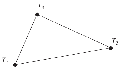
Compute element stiffness matrix for a triangular heat flow element.

Syntax:

Ke = flw2te(ex, ey, ep, D)
[Ke, fe] = flw2te(ex, ey, ep, D, eq)

Description:

flw2te provides the element stiffness (conductivity) matrix Ke and the element load vector fe for a triangular heat flow element.

The element nodal coordinates \(x_1\), \(y_1\), \(x_2\) etc, are supplied to the function by ex and ey, the element thickness \(t\) is supplied by ep and the thermal conductivities (or corresponding quantities) \(k_{xx}\), \(k_{xy}\) etc are supplied by D.

\[\begin{split}\begin{array}{l} \mathbf{ex} = [\, x_1 \;\; x_2 \;\; x_3\,] \\ \mathbf{ey} = [\, y_1 \;\; y_2 \;\; y_3\,] \end{array} \qquad \mathbf{ep} = [\, t \,] \qquad \mathbf{D} = \begin{bmatrix} k_{xx} & k_{xy} \\ k_{yx} & k_{yy} \end{bmatrix}\end{split}\]

If the scalar variable eq is given in the function, the element load vector \(\mathbf{fe}\) is computed, using

\[\mathbf{eq} = [\, Q \,]\]

where \(Q\) is the heat supply per unit volume.

Theory:

The element stiffness matrix \(\mathbf{K}^e\) and the element load vector \(\mathbf{f}_l^e\), stored in Ke and fe, respectively, are computed according to

\[\mathbf{K}^e = (\mathbf{C}^{-1})^T \int_A \bar{\mathbf{B}}^T \mathbf{D} \bar{\mathbf{B}}\, t\, dA\, \mathbf{C}^{-1}\]

\[\mathbf{f}_l^e = (\mathbf{C}^{-1})^T \int_A \bar{\mathbf{N}}^T Q\, t\, dA\]

with the constitutive matrix \(\mathbf{D}\) defined by D.

The evaluation of the integrals for the triangular element is based on the linear temperature approximation \(T(x, y)\) and is expressed in terms of the nodal variables \(T_1\), \(T_2\) and \(T_3\) as

\[T(x, y) = \mathbf{N}^e \mathbf{a}^e = \bar{\mathbf{N}}\, \mathbf{C}^{-1} \mathbf{a}^e\]

where

\[\begin{split}\bar{\mathbf{N}} = [\, 1 \;\; x \;\; y\,] \qquad \mathbf{C} = \begin{bmatrix} 1 & x_1 & y_1 \\ 1 & x_2 & y_2 \\ 1 & x_3 & y_3 \end{bmatrix} \qquad \mathbf{a}^e = \begin{bmatrix} T_1 \\ T_2 \\ T_3 \end{bmatrix}\end{split}\]

and hence it follows that

\[\begin{split}\bar{\mathbf{B}} = \nabla \bar{\mathbf{N}} = \begin{bmatrix} 0 & 1 & 0 \\ 0 & 0 & 1 \end{bmatrix} \qquad \nabla = \begin{bmatrix} \dfrac{\partial}{\partial x} \\ \dfrac{\partial}{\partial y} \end{bmatrix}\end{split}\]

Evaluation of the integrals for the triangular element yields

\[\mathbf{K}^e = (\mathbf{C}^{-1})^T \bar{\mathbf{B}}^T \mathbf{D} \bar{\mathbf{B}} \mathbf{C}^{-1} t A\]

\[\begin{split}\mathbf{f}_l^e = \frac{Q A t}{3} \begin{bmatrix} 1 \\ 1 \\ 1 \end{bmatrix}\end{split}\]

where the element area \(A\) is determined as

\[A = \frac{1}{2} \det \mathbf{C}\]

flw2ts¶

Purpose:

Compute heat flux and temperature gradients in a triangular heat flow element.

Syntax:

[es, et] = flw2ts(ex, ey, D, ed)

Description:

flw2ts computes the heat flux vector es and the temperature gradient et (or corresponding quantities) in a triangular heat flow element.

The input variables ex, ey and the matrix D are defined in flw2te. The vector ed contains the nodal temperatures \(\mathbf{a}^e\) of the element and is obtained by the function extract as

\[\mathbf{ed} = (\mathbf{a}^e)^T = [\;T_1\;\; T_2\;\; T_3\;]\]

The output variables

\[\mathbf{es} = \mathbf{q}^T = \left[\; q_x \; q_y \;\right]\]

\[\mathbf{et} = (\nabla T)^T = \left[\begin{array}{l} \frac{\partial T}{\partial x}\;\;\frac{\partial T}{\partial y} \end{array} \right]\]

contain the components of the heat flux and the temperature gradient computed in the directions of the coordinate axis.

Theory:

The temperature gradient and the heat flux are computed according to

\[\nabla T = \bar{\mathbf{B}}\;\mathbf{C}^{-1}\;\mathbf{a}^e\]

\[\mathbf{q} = - \mathbf{D} \nabla T\]

where the matrices \(\mathbf{D}\), \(\bar{\mathbf{B}}\), and \(\mathbf{C}\) are described in flw2te. Note that both the temperature gradient and the heat flux are constant in the element.

flw2qe¶

Purpose:

Compute element stiffness matrix for a quadrilateral heat flow element.

Syntax:

Ke = flw2qe(ex, ey, ep, D)
[Ke, fe] = flw2qe(ex, ey, ep, D, eq)

Description:

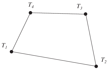
flw2qe provides the element stiffness (conductivity) matrix Ke and the element load vector fe for a quadrilateral heat flow element.

The element nodal coordinates \(x_1\), \(y_1\), \(x_2\) etc, are supplied to the function by ex and ey, the element thickness \(t\) is supplied by ep and the thermal conductivities (or corresponding quantities) \(k_{xx}\), \(k_{xy}\) etc are supplied by D.

\[\begin{split}\begin{array}{l} \mathbf{ex} = [\, x_1 \;\; x_2 \;\; x_3 \;\; x_4 \,] \\ \mathbf{ey} = [\, y_1 \;\; y_2 \;\; y_3 \;\; y_4 \,] \end{array} \qquad \mathbf{ep} = \left[\, t \,\right] \qquad \mathbf{D} = \left[ \begin{array}{cc} k_{xx} & k_{xy} \\ k_{yx} & k_{yy} \end{array} \right]\end{split}\]

If the scalar variable eq is given in the function, the element load vector \(\mathbf{fe}\) is computed, using

\[\mathbf{eq} = \left[\, Q \,\right]\]

where \(Q\) is the heat supply per unit volume.

Theory:

In computing the element matrices, a fifth degree of freedom is introduced. The location of this extra degree of freedom is defined by the mean value of the coordinates in the corner points. Four sets of element matrices are calculated using flw2te. These matrices are then assembled and the fifth degree of freedom is eliminated by static condensation.

flw2qs¶

Purpose:

Compute heat flux and temperature gradients in a quadrilateral heat flow element.

Syntax:

[es, et] = flw2qs(ex, ey, ep, D, ed)
[es, et] = flw2qs(ex, ey, ep, D, ed, eq)

Description:

flw2qs computes the heat flux vector es and the temperature gradient et (or corresponding quantities) in a quadrilateral heat flow element.

The input variables ex, ey, eq and the matrix D are defined in flw2qe. The vector ed contains the nodal temperatures \(\mathbf{a}^e\) of the element and is obtained by the function extract as

\[\mathbf{ed} = (\mathbf{a}^e)^T = [\;T_1\;\; T_2\;\; T_3\;\; T_4\;]\]

The output variables

\[\mathbf{es} = \mathbf{q}^T = \left[\; q_x \; q_y \;\right]\]

\[\mathbf{et} = (\nabla T)^T = \left[\begin{array}{l} \frac{\partial T}{\partial x}\;\;\frac{\partial T}{\partial y} \end{array} \right]\]

contain the components of the heat flux and the temperature gradient computed in the directions of the coordinate axis.

Theory:

By assembling four triangular elements as described in flw2te a system of equations containing 5 degrees of freedom is obtained. From this system of equations the unknown temperature at the center of the element is computed. Then according to the description in flw2ts the temperature gradient and the heat flux in each of the four triangular elements are produced. Finally the temperature gradient and the heat flux of the quadrilateral element are computed as area weighted mean values from the values of the four triangular elements. If heat is supplied to the element, the element load vector eq is needed for the calculations.

Note

If the input variables are given for a number of identical (nie) elements, i.e. Ex, Ey, and Ed are matrices, then the output variables are defined as

\[\begin{split}\mathrm{Es} = \left[ \begin{array}{cc} q^1_x & q^1_y \\ q^2_x & q^2_y \\ \vdots & \vdots \\ q^{nie}_x & q^{nie}_y \end{array} \right] \qquad \mathrm{Et} = \left[ \begin{array}{cc} \frac{\partial T}{\partial x}^1 & \frac{\partial T}{\partial y}^1 \\ \frac{\partial T}{\partial x}^2 & \frac{\partial T}{\partial y}^2 \\ \vdots & \vdots \\ \frac{\partial T}{\partial x}^{nie} & \frac{\partial T}{\partial y}^{nie} \end{array} \right]\end{split}\]

where \(\mathbf{q}^i\) and \(\nabla T^i\) are computed from the nodal values located in column i of Ed.

flw2i4e¶

Purpose:

Compute element stiffness matrix for a 4 node isoparametric heat flow element.

Syntax:

Ke = flw2i4e(ex, ey, ep, D)
[Ke, fe] = flw2i4e(ex, ey, ep, D, eq)

Description:

flw2i4e provides the element stiffness (conductivity) matrix Ke and the element load vector fe for a 4 node isoparametric heat flow element.

The element nodal coordinates \(x_1\), \(y_1\), \(x_2\) etc, are supplied to the function by ex and ey. The element thickness \(t\) and the number of Gauss points \(n\) (\(n \times n\) integration points, \(n=1,2,3\)) are supplied to the function by ep and the thermal conductivities (or corresponding quantities) \(k_{xx}\), \(k_{xy}\) etc are supplied by D.

\[\begin{split}\begin{array}{l} \mathbf{ex} = [\, x_1 \;\; x_2 \;\; x_3 \;\; x_4 \,] \\ \mathbf{ey} = [\, y_1 \;\; y_2 \;\; y_3 \;\; y_4 \,] \end{array} \qquad \mathbf{ep} = [\, t \;\; n \,] \qquad \mathbf{D} = \begin{bmatrix} k_{xx} & k_{xy} \\ k_{yx} & k_{yy} \end{bmatrix}\end{split}\]

If the scalar variable eq is given in the function, the element load vector \(fe\) is computed, using

\[\mathbf{eq} = [\, Q \,]\]

where \(Q\) is the heat supply per unit volume.

Theory:

The element stiffness matrix \(\mathbf{K}^e\) and the element load vector \(\mathbf{f}_l^e\), stored in Ke and fe, respectively, are computed according to

\[\mathbf{K}^e = \int_A \mathbf{B}^{eT} \mathbf{D} \mathbf{B}^e t\, dA\]

\[\mathbf{f}_l^e = \int_A \mathbf{N}^{eT} Q t\, dA\]

with the constitutive matrix \(\mathbf{D}\) defined by D.

The evaluation of the integrals for the isoparametric 4 node element is based on a temperature approximation \(T(\xi, \eta)\), expressed in a local coordinate system in terms of the nodal variables \(T_1\), \(T_2\), \(T_3\) and \(T_4\) as

\[T(\xi, \eta) = \mathbf{N}^e \mathbf{a}^e\]

where

\[\mathbf{N}^e = [\, N_1^e \;\; N_2^e \;\; N_3^e \;\; N_4^e \,] \qquad \mathbf{a}^e = [\, T_1 \;\; T_2 \;\; T_3 \;\; T_4 \,]^T\]

The element shape functions are given by

\[\begin{split}N_1^e = \frac{1}{4}(1-\xi)(1-\eta) \qquad N_2^e = \frac{1}{4}(1+\xi)(1-\eta) \\ N_3^e = \frac{1}{4}(1+\xi)(1+\eta) \qquad N_4^e = \frac{1}{4}(1-\xi)(1+\eta)\end{split}\]

The \(\mathbf{B}^e\)-matrix is given by

\[\begin{split}\mathbf{B}^e = \nabla \mathbf{N}^e = \begin{bmatrix} \frac{\partial}{\partial x} \\ \frac{\partial}{\partial y} \end{bmatrix} \mathbf{N}^e = (\mathbf{J}^T)^{-1} \begin{bmatrix} \frac{\partial}{\partial \xi} \\ \frac{\partial}{\partial \eta} \end{bmatrix} \mathbf{N}^e\end{split}\]

where \(\mathbf{J}\) is the Jacobian matrix

\[\begin{split}\mathbf{J} = \begin{bmatrix} \frac{\partial x}{\partial \xi} & \frac{\partial x}{\partial \eta} \\ \frac{\partial y}{\partial \xi} & \frac{\partial y}{\partial \eta} \end{bmatrix}\end{split}\]

Evaluation of the integrals is done by Gauss integration.

flw2i4s¶

Purpose:

Compute heat flux and temperature gradients in a 4 node isoparametric heat flow element.

Syntax:

[es, et, eci] = flw2i4s(ex, ey, ep, D, ed)

Description:

flw2i4s computes the heat flux vector es and the temperature gradient et (or corresponding quantities) in a 4 node isoparametric heat flow element.

The input variables \(\mathbf{ex}\), \(\mathbf{ey}\), \(\mathbf{ep}\) and the matrix \(\mathbf{D}\) are defined in flw2i4e. The vector \(\mathbf{ed}\) contains the nodal temperatures \(\mathbf{a}^e\) of the element and is obtained by extract as

\[\mathbf{ed} = (\mathbf{a}^e)^T = [\;T_1\;\; T_2\;\; T_3\;\; T_4\;]\]

The output variables

\[\begin{split}\mathbf{es} = \bar{\mathbf{q}}^T = \left[ \begin{array}{cc} q^1_x & q^1_y \\ q^2_x & q^2_y \\ \vdots & \vdots \\ q^{n^2}_x & q^{n^2}_y \end{array} \right]\end{split}\]

\[ \begin{align}\begin{aligned}\begin{split}\mathbf{et} = (\bar {\nabla} T)^T = \left[ \begin{array}{cc} \frac{\partial T}{\partial x}^1 & \frac{\partial T}{\partial y}^1 \\ \frac{\partial T}{\partial x}^2 & \frac{\partial T}{\partial y}^2 \\ \vdots & \vdots \\ \frac{\partial T}{\partial x}^{n^2} & \frac{\partial T}{\partial y}^{n^2} \end{array} \right]\end{split}\\\begin{split}\qquad \mathbf{eci} = \left[ \begin{array}{cc} x_1 & y_1 \\ x_2 & y_2 \\ \vdots & \vdots \\ x_{n^2} & y_{n^2} \end{array} \right]\end{split}\end{aligned}\end{align} \]

contain the heat flux, the temperature gradient, and the coordinates of the integration points. The index \(n\) denotes the number of integration points used within the element, cf. flw2i4e.

Theory:

The temperature gradient and the heat flux are computed according to

\[\nabla T = \mathbf{B}^e\,\mathbf{a}^e\]

\[\mathbf{q} = - \mathbf{D} \nabla T\]

where the matrices \(\mathbf{D}\), \(\mathbf{B}^e\), and \(\mathbf{a}^e\) are described in flw2i4e, and where the integration points are chosen as evaluation points.

flw2i8e¶

Purpose:

Compute element stiffness matrix for an 8 node isoparametric heat flow element.

Syntax:

Ke = flw2i8e(ex, ey, ep, D)
[Ke, fe] = flw2i8e(ex, ey, ep, D, eq)

Description:

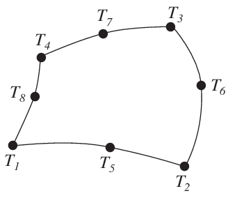
flw2i8e provides the element stiffness (conductivity) matrix Ke and the element load vector fe for an 8 node isoparametric heat flow element.

The element nodal coordinates \(x_1\), \(y_1\), \(x_2\) etc, are supplied to the function by \(\mathbf{ex}\) and \(\mathbf{ey}\). The element thickness \(t\) and the number of Gauss points \(n\) (\(n \times n\) integration points, \(n=1,2,3\)) are supplied to the function by \(\mathbf{ep}\) and the thermal conductivities (or corresponding quantities) \(k_{xx}\), \(k_{xy}\) etc are supplied by D.

\[\begin{split}\begin{array}{l} \mathbf{ex} = [\, x_1 \;\; x_2 \;\; x_3 \;\; \dots \;\; x_8 \,] \\ \mathbf{ey} = [\, y_1 \;\; y_2 \;\; y_3 \;\; \dots \;\; y_8 \,] \end{array} \qquad \mathbf{ep} = [\, t \;\; n \,] \qquad \mathbf{D} = \begin{bmatrix} k_{xx} & k_{xy} \\ k_{yx} & k_{yy} \end{bmatrix}\end{split}\]

If the scalar variable eq is given in the function, the vector \(\mathbf{fe}\) is computed, using

\[\mathbf{eq} = [\, Q \,]\]

where \(Q\) is the heat supply per unit volume.

Theory:

The element stiffness matrix \(\mathbf{K}^e\) and the element load vector \(\mathbf{f}_l^e\), stored in Ke and fe, respectively, are computed according to

\[\mathbf{K}^e = \int_A \mathbf{B}^{eT} \mathbf{D} \mathbf{B}^e t\, dA\]

\[\mathbf{f}_l^e = \int_A \mathbf{N}^{eT} Q t\, dA\]

with the constitutive matrix \(\mathbf{D}\) defined by D.

The evaluation of the integrals for the 2D isoparametric 8 node element is based on a temperature approximation \(T(\xi, \eta)\), expressed in a local coordinates system in terms of the nodal variables \(T_1\) to \(T_8\) as

\[T(\xi, \eta) = \mathbf{N}^e \mathbf{a}^e\]

where

\[\mathbf{N}^e = [\, N_1^e \;\; N_2^e \;\; N_3^e \;\; \dots \;\; N_8^e \,] \qquad \mathbf{a}^e = [\, T_1 \;\; T_2 \;\; T_3 \;\; \dots \;\; T_8 \,]^T\]

The element shape functions are given by

\[\begin{split}\begin{aligned} N_1^e &= -\frac{1}{4}(1-\xi)(1-\eta)(1+\xi+\eta) & N_5^e &= \frac{1}{2}(1-\xi^2)(1-\eta) \\ N_2^e &= -\frac{1}{4}(1+\xi)(1-\eta)(1-\xi+\eta) & N_6^e &= \frac{1}{2}(1+\xi)(1-\eta^2) \\ N_3^e &= -\frac{1}{4}(1+\xi)(1+\eta)(1-\xi-\eta) & N_7^e &= \frac{1}{2}(1-\xi^2)(1+\eta) \\ N_4^e &= -\frac{1}{4}(1-\xi)(1+\eta)(1+\xi-\eta) & N_8^e &= \frac{1}{2}(1-\xi)(1-\eta^2) \end{aligned}\end{split}\]

The \(\mathbf{B}^e\)-matrix is given by

\[\begin{split}\mathbf{B}^e = \nabla \mathbf{N}^e = \begin{bmatrix} \frac{\partial}{\partial x} \\ \frac{\partial}{\partial y} \end{bmatrix} \mathbf{N}^e = (\mathbf{J}^T)^{-1} \begin{bmatrix} \frac{\partial}{\partial \xi} \\ \frac{\partial}{\partial \eta} \end{bmatrix} \mathbf{N}^e\end{split}\]

where \(\mathbf{J}\) is the Jacobian matrix

\[\begin{split}\mathbf{J} = \begin{bmatrix} \frac{\partial x}{\partial \xi} & \frac{\partial x}{\partial \eta} \\ \frac{\partial y}{\partial \xi} & \frac{\partial y}{\partial \eta} \end{bmatrix}\end{split}\]

Evaluation of the integrals is done by Gauss integration.

flw2i8s¶

Purpose:

Compute heat flux and temperature gradients in an 8 node isoparametric heat flow element.

Syntax:

[es, et, eci] = flw2i8s(ex, ey, ep, D, ed)

Description:

flw2i8s computes the heat flux vector es and the temperature gradient et (or corresponding quantities) in an 8 node isoparametric heat flow element.

The input variables ex, ey, ep and the matrix D are defined in flw2i8e. The vector ed contains the nodal temperatures \(\mathbf{a}^e\) of the element and is obtained by the function extract as

\[\mathbf{ed} = (\mathbf{a}^e)^T = [\;T_1\;\; T_2\;\; T_3\;\;\dots\;\, T_8\;]\]

The output variables

\[\begin{split}\mathbf{es} = \bar{\mathbf{q}}^T = \left[ \begin{array}{cc} q^1_x & q^1_y \\ q^2_x & q^2_y \\ \vdots & \vdots \\ q^{n^2}_x & q^{n^2}_y \end{array} \right]\end{split}\]

\[\begin{split}\mathbf{et} = (\bar {\nabla} T)^T = \left[ \begin{array}{cc} \frac{\partial T}{\partial x}^1 & \frac{\partial T}{\partial y}^1 \\ \frac{\partial T}{\partial x}^2 & \frac{\partial T}{\partial y}^2 \\ \vdots & \vdots \\ \frac{\partial T}{\partial x}^{n^2} & \frac{\partial T}{\partial y}^{n^2} \end{array} \right]\end{split}\]

\[\begin{split}\mathbf{eci} = \left[ \begin{array}{cc} x_1 & y_1 \\ x_2 & y_2 \\ \vdots & \vdots \\ x_{n^2} & y_{n^2} \end{array} \right]\end{split}\]

contain the heat flux, the temperature gradient, and the coordinates of the integration points. The index \(n\) denotes the number of integration points used within the element, see flw2i8e.

Theory:

The temperature gradient and the heat flux are computed according to

\[\nabla T = \mathbf{B}^e\,\mathbf{a}^e\]

\[\mathbf{q} = - \mathbf{D} \nabla T\]

where the matrices \(\mathbf{D}\), \(\mathbf{B}^e\), and \(\mathbf{a}^e\) are described in flw2i8e, and where the integration points are chosen as evaluation points.

flw3i8e¶

Purpose:

Compute element stiffness matrix for an 8 node isoparametric element.

Syntax:

Ke = flw3i8e(ex, ey, ez, ep, D)
[Ke, fe] = flw3i8e(ex, ey, ez, ep, D, eq)

Description:

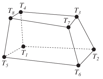
flw3i8e provides the element stiffness (conductivity) matrix Ke and the element load vector fe for an 8 node isoparametric heat flow element.

The element nodal coordinates \(x_1\), \(y_1\), \(z_1\), \(x_2\) etc, are supplied to the function by ex, ey and ez. The number of Gauss points \(n\) (\(n \times n \times n\) integration points, \(n=1,2,3\)) are supplied to the function by ep and the thermal conductivities (or corresponding quantities) \(k_{xx}\), \(k_{xy}\) etc are supplied by D.

\[\begin{split}\begin{array}{l} \mathbf{ex} = [\, x_1 \;\; x_2 \;\; x_3 \;\; \dots \;\; x_8 \,] \\ \mathbf{ey} = [\, y_1 \;\; y_2 \;\; y_3 \;\; \dots \;\; y_8 \,] \\ \mathbf{ez} = [\, z_1 \;\; z_2 \;\; z_3 \;\; \dots \;\; z_8 \,] \end{array} \qquad \mathbf{ep} = [\, n \,] \qquad \mathbf{D} = \begin{bmatrix} k_{xx} & k_{xy} & k_{xz} \\ k_{yx} & k_{yy} & k_{yz} \\ k_{zx} & k_{zy} & k_{zz} \end{bmatrix}\end{split}\]

If the scalar variable eq is given in the function, the element load vector \(\mathbf{fe}\) is computed, using

\[\mathbf{eq} = [\, Q \,]\]

where \(Q\) is the heat supply per unit volume.

Theory:

The element stiffness matrix \(\mathbf{K}^e\) and the element load vector \(\mathbf{f}_l^e\), stored in Ke and fe, respectively, are computed according to

\[ \begin{align}\begin{aligned}\mathbf{K}^e = \int_V \mathbf{B}^{eT} \mathbf{D} \mathbf{B}^e \, dV\\\mathbf{f}_l^e = \int_V \mathbf{N}^{eT} Q \, dV\end{aligned}\end{align} \]

with the constitutive matrix \(\mathbf{D}\) defined by D.

The evaluation of the integrals for the 3D isoparametric 8 node element is based on a temperature approximation \(T(\xi, \eta, \zeta)\), expressed in a local coordinate system in terms of the nodal variables \(T_1\) to \(T_8\) as

\[ \begin{align}\begin{aligned}T(\xi, \eta, \zeta) = \mathbf{N}^e \mathbf{a}^e\\\mathbf{N}^e = [\, N_1^e \;\; N_2^e \;\; N_3^e \;\; \dots \;\; N_8^e \,] \qquad \mathbf{a}^e = [\, T_1 \;\; T_2 \;\; T_3 \;\; \dots \;\; T_8 \,]^T\end{aligned}\end{align} \]

The element shape functions are given by

\[\begin{split}N_1^e = \frac{1}{8}(1-\xi)(1-\eta)(1-\zeta) \qquad N_2^e = \frac{1}{8}(1+\xi)(1-\eta)(1-\zeta) \\ N_3^e = \frac{1}{8}(1+\xi)(1+\eta)(1-\zeta) \qquad N_4^e = \frac{1}{8}(1-\xi)(1+\eta)(1-\zeta) \\ N_5^e = \frac{1}{8}(1-\xi)(1-\eta)(1+\zeta) \qquad N_6^e = \frac{1}{8}(1+\xi)(1-\eta)(1+\zeta) \\ N_7^e = \frac{1}{8}(1+\xi)(1+\eta)(1+\zeta) \qquad N_8^e = \frac{1}{8}(1-\xi)(1+\eta)(1+\zeta)\end{split}\]

The \(\mathbf{B}^e\)-matrix is given by

\[\begin{split}\mathbf{B}^e = \nabla \mathbf{N}^e = \begin{bmatrix} \frac{\partial}{\partial x} \\ \frac{\partial}{\partial y} \\ \frac{\partial}{\partial z} \end{bmatrix} \mathbf{N}^e = (\mathbf{J}^T)^{-1} \begin{bmatrix} \frac{\partial}{\partial \xi} \\ \frac{\partial}{\partial \eta} \\ \frac{\partial}{\partial \zeta} \end{bmatrix} \mathbf{N}^e\end{split}\]

where \(\mathbf{J}\) is the Jacobian matrix

\[\begin{split}\mathbf{J} = \begin{bmatrix} \frac{\partial x}{\partial \xi} & \frac{\partial x}{\partial \eta} & \frac{\partial x}{\partial \zeta} \\ \frac{\partial y}{\partial \xi} & \frac{\partial y}{\partial \eta} & \frac{\partial y}{\partial \zeta} \\ \frac{\partial z}{\partial \xi} & \frac{\partial z}{\partial \eta} & \frac{\partial z}{\partial \zeta} \end{bmatrix}\end{split}\]

Evaluation of the integrals is done by Gauss integration.

flw3i8s¶

Purpose:

Compute heat flux and temperature gradients in an 8 node isoparametric heat flow element.

Syntax:

[es, et, eci] = flw3i8s(ex, ey, ez, ep, D, ed)

Description:

flw3i8s computes the heat flux vector es and the temperature gradient et (or corresponding quantities) in an 8 node isoparametric heat flow element.

The input variables \(\mathbf{ex}\), \(\mathbf{ey}\), \(\mathbf{ez}\), \(\mathbf{ep}\) and the matrix \(\mathbf{D}\) are defined in flw3i8e. The vector \(\mathbf{ed}\) contains the nodal temperatures \(\mathbf{a}^e\) of the element and is obtained by the function extract as

\[\mathbf{ed} = (\mathbf{a}^e)^T = [\,T_1\;\; T_2\;\; T_3\;\;\dots\;\; T_8\,]\]

The output variables

\[\begin{split}\mathbf{es} = \bar{\mathbf{q}}^T = \begin{bmatrix} q^1_x & q^1_y & q^1_z \\ q^2_x & q^2_y & q^2_z \\ \vdots & \vdots & \vdots\\ q^{n^3}_x & q^{n^3}_y & q^{n^3}_z \end{bmatrix}\end{split}\]

\[\begin{split}\mathbf{et} = (\bar {\nabla} T)^T = \begin{bmatrix} \frac{\partial T}{\partial x}^1 & \frac{\partial T}{\partial y}^1 & \frac{\partial T}{\partial z}^1\\ \frac{\partial T}{\partial x}^2 & \frac{\partial T}{\partial y}^2 & \frac{\partial T}{\partial z}^2\\ \vdots & \vdots & \vdots \\ \frac{\partial T}{\partial x}^{n^3} & \frac{\partial T}{\partial y}^{n^3} & \frac{\partial T}{\partial z}^{n^3} \end{bmatrix} \qquad \mathbf{eci} = \begin{bmatrix} x_1 & y_1 & z_1 \\ x_2 & y_2 & z_2 \\ \vdots & \vdots & \vdots \\ x_{n^3} & y_{n^3} & z_{n^3} \end{bmatrix}\end{split}\]

contain the heat flux, the temperature gradient, and the coordinates of the integration points. The index \(n\) denotes the number of integration points used within the element, see flw3i8e.

Theory:

The temperature gradient and the heat flux are computed according to

\[\nabla T = \mathbf{B}^e\,\mathbf{a}^e\]

\[\mathbf{q} = - \mathbf{D} \nabla T\]

where the matrices \(\mathbf{D}\), \(\mathbf{B}^e\), and \(\mathbf{a}^e\) are described in flw3i8e, and where the integration points are chosen as evaluation points.