Examples¶

exs_spring¶

Purpose:

Show the basic steps in a finite element calculation.

Description:

The general procedure in linear finite element calculations is carried out for a simple structure. The steps are:

Define the model
Generate element matrices
Assemble element matrices into the global system of equations
Solve the global system of equations
Evaluate element forces

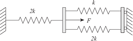
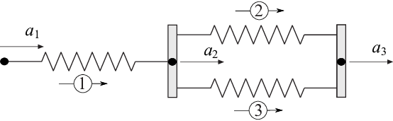
Consider the system of three linear elastic springs, and the corresponding finite element model. The system of springs is fixed in its ends and loaded by a single load \(F\).

Example:

The computation is initialized by defining the topology matrix Edof, containing element numbers and global element degrees of freedom:

>> Edof=[1  1 2;
         2  2 3;
         3  2 3];

The global stiffness matrix K (3×3) of zeros:

>> K=zeros(3,3)

K =
     0     0     0
     0     0     0
     0     0     0

And the load vector f (3×1) with the load \(F=100\) in position 2:

>> f=zeros(3,1);  f(2)=100

f =
      0
    100
      0

Element stiffness matrices are generated by the function spring1e. The element property ep for the springs contains the spring stiffnesses \(k\) and \(2k\) respectively, where \(k=1500\):

>> k=1500;  ep1=2*k;  ep2=k;  ep3=2*k;
>> Ke1=spring1e(ep1)

Ke1 =
        3000       -3000
       -3000        3000

>> Ke2=spring1e(ep2)

Ke2 =
        1500       -1500
       -1500        1500

>> Ke3=spring1e(ep3)

Ke1 =
        3000       -3000
       -3000        3000

The element stiffness matrices are assembled into the global stiffness matrix K according to the topology:

>> K=assem(Edof(1,:),K,Ke1)

K =
        3000       -3000           0
       -3000        3000           0
           0           0           0

>> K=assem(Edof(2,:),K,Ke2)

K =
        3000       -3000           0
       -3000        4500       -1500
           0       -1500        1500

>> K=assem(Edof(3,:),K,Ke3)

K =
        3000       -3000           0
       -3000        7500       -4500
           0       -4500        4500

The global system of equations is solved considering the boundary conditions given in bc:

>> bc= [1 0; 3 0];
>> [a,r]=solveq(K,f,bc)

a =
         0
    0.0133
         0

r =

  -40.0000
         0
  -60.0000

Element forces are evaluated from the element displacements. These are obtained from the global displacements a using the function extract:

>> ed1=extract_ed(Edof(1,:),a)

ed1 =
      0      0.0133

>> ed2=extract_ed(Edof(2,:),a)

ed2 =
      0.0133      0

>> ed3=extract_ed(Edof(3,:),a)

ed3 =
      0.0133      0

The spring forces are evaluated using the function spring1s:

>> es1=spring1s(ep1,ed1)

es1 =
       40

>> es2=spring1s(ep2,ed2)

es2 =
      -20

>> es3=spring1s(ep3,ed3)

es3 =
      -40

exs_flw_temp1¶

Purpose:

Analysis of one-dimensional heat flow.

Description:

Consider a wall built up of concrete and thermal insulation. The outdoor temperature is \(-17°\text{C}\) and the temperature inside is \(20°\text{C}\). At the inside of the thermal insulation there is a heat source yielding \(10\) W/m².

The wall is subdivided into five elements and the one-dimensional spring (analogy) element spring1e is used. Equivalent spring stiffnesses are \(k_i=\lambda A/L\) for thermal conductivity and \(k_i=A/R\) for thermal surface resistance. Corresponding spring stiffnesses per m² of the wall are:

\(k_1 =\)	\(1/0.04\)	\(=\)	\(25.0\)	W/K
\(k_2 =\)	\(1.7/0.070\)	\(=\)	\(24.3\)	W/K
\(k_3 =\)	\(0.040/0.100\)	\(=\)	\(0.4\)	W/K
\(k_4 =\)	\(1.7/0.100\)	\(=\)	\(17.0\)	W/K
\(k_5 =\)	\(1/0.13\)	\(=\)	\(7.7\)	W/K

Example:

A global system matrix K and a heat flow vector f are defined. The heat source inside the wall is considered by setting \(f_4=10\). The element matrices Ke are computed using spring1e, and the function assem assembles the global stiffness matrix.

The system of equations is solved using solveq with considerations to the boundary conditions in bc. The prescribed temperatures are \(a_1=-17°\text{C}\) and \(a_6=20°\text{C}\).

>> Edof=[1  1 2
         2  2 3;
         3  3 4;
         4  4 5;
         5  5 6];

>> K=zeros(6);
>> f=zeros(6,1);  f(4)=10

f =

     0
     0
     0
    10
     0
     0

>> ep1=[25];  ep2=[24.3];
>> ep3=[0.4];  ep4=[17];
>> ep5=[7.7];

>> Ke1=spring1e(ep1);       Ke2=spring1e(ep2);
>> Ke3=spring1e(ep3);       Ke4=spring1e(ep4);
>> Ke5=spring1e(ep5);

>> K=assem(Edof(1,:),K,Ke1);   K=assem(Edof(2,:),K,Ke2);
>> K=assem(Edof(3,:),K,Ke3);   K=assem(Edof(4,:),K,Ke4);
>> K=assem(Edof(5,:),K,Ke5);

>> bc=[1 -17; 6 20];

>> [a,r]=solveq(K,f,bc)

a =

  -17.0000
  -16.4384
  -15.8607
   19.2378
   19.4754
   20.0000

r =

  -14.0394
    0.0000
   -0.0000
   -0.0000
         0
    0.0000
    4.0394

The temperature values \(a_i\) in the node points are given in the vector a and the boundary flows in the vector r.

After solving the system of equations, the heat flow through the wall is computed using extract and spring1s:

>> ed1=extract_ed(Edof(1,:),a);
>> ed2=extract_ed(Edof(2,:),a);
>> ed3=extract_ed(Edof(3,:),a);
>> ed4=extract_ed(Edof(4,:),a);
>> ed5=extract_ed(Edof(5,:),a);

>> q1=spring1s(ep1,ed1)

q1 =

   14.0394

>> q2=spring1s(ep2,ed2)

q2 =

   14.0394

>> q3=spring1s(ep3,ed3)

q3 =

   14.0394

>> q4=spring1s(ep4,ed4)

q4 =

    4.0394

>> q5=spring1s(ep5,ed5)

q5 =

    4.0394

The heat flow through the wall is \(q=14.0\) W/m² in the part of the wall to the left of the heat source, and \(q=4.0\) W/m² in the part to the right of the heat source.

exs_bar2¶

Purpose:

Analysis of a plane truss.

Description:

Consider a plane truss consisting of three bars with the properties \(E=200\) GPa, \(A_1=6.0 \times 10^{-4}\) m², \(A_2=3.0 \times 10^{-4}\) m² and \(A_3=10.0 \times 10^{-4}\) m², and loaded by a single force \(P=80\) kN. The corresponding finite element model consists of three elements and eight degrees of freedom.

Example:

The topology is defined by the matrix:

>> Edof=[1   1  2  5  6;
         2   5  6  7  8;
         3   3  4  5  6];

The stiffness matrix K and the load vector f, are defined by:

>> K=zeros(8);
   f=zeros(8,1); f(6)=-80e3;

The element property vectors ep1, ep2 and ep3 are defined by:

>> E=2.0e11;
>> A1=6.0e-4;     A2=3.0e-4;     A3=10.0e-4;
>> ep1=[E A1];    ep2=[E A2];    ep3=[E A3];

And the element coordinate vectors ex1, ex2, ex3, ey1, ey2 and ey3 by:

>> ex1=[0 1.6];    ex2=[1.6 1.6];    ex3=[0 1.6];
>> ey1=[0 0];      ey2=[0 1.2];      ey3=[1.2 0];

The element stiffness matrices Ke1, Ke2 and Ke3 are computed using bar2e:

>> Ke1=bar2e(ex1,ey1,ep1)

Ke1 =

  1.0e+007 *

    7.5000         0   -7.5000         0
         0         0         0         0
   -7.5000         0    7.5000         0
         0         0         0         0

>> Ke2=bar2e(ex2,ey2,ep2)

Ke2 =

  1.0e+007 *

         0         0         0         0
         0    5.0000         0   -5.0000
         0         0         0         0
         0   -5.0000         0    5.0000

>> Ke3=bar2e(ex3,ey3,ep3)

Ke3 =

  1.0e+007 *

    6.4000   -4.8000   -6.4000    4.8000
   -4.8000    3.6000    4.8000   -3.6000
   -6.4000    4.8000    6.4000   -4.8000
    4.8000   -3.6000   -4.8000    3.6000

Based on the topology information, the global stiffness matrix can be generated by assembling the element stiffness matrices:

>> K=assem(Edof(1,:),K,Ke1);
>> K=assem(Edof(2,:),K,Ke2);
>> K=assem(Edof(3,:),K,Ke3)

K =

  1.0e+008 *

  Columns 1 through 7

    0.7500         0         0         0   -0.7500         0         0
         0         0         0         0         0         0         0
         0         0    0.6400   -0.4800   -0.6400    0.4800         0
         0         0   -0.4800    0.3600    0.4800   -0.3600         0
   -0.7500         0   -0.6400    0.4800    1.3900   -0.4800         0
         0         0    0.4800   -0.3600   -0.4800    0.8600         0
         0         0         0         0         0         0         0
         0         0         0         0         0   -0.5000         0

  Column 8

         0
         0
         0
         0
         0
   -0.5000
         0
    0.5000

Considering the prescribed displacements in bc, the system of equations is solved using the function solveq, yielding displacements a and support forces r:

>> bc= [1 0;2 0;3 0;4 0;7 0;8 0];
>> [a,r]=solveq(K,f,bc)

a =

  1.0e-002 *

         0
         0
         0
         0
   -0.0398
   -0.1152
         0
         0

r =

  1.0e+004 *

    2.9845
         0
   -2.9845
    2.2383
    0.0000
    0.0000
         0
    5.7617

The vertical displacement at the point of loading is 1.15 mm. The section forces es1, es2 and es3 are calculated using bar2s from element displacements ed1, ed2 and ed3 obtained using extract:

>> ed1=extract_ed(Edof(1,:),a);
>> es1=bar2s(ex1,ey1,ep1,ed1)

es1 =

  1.0e+004 *

   -2.9845
   -2.9845

>> ed2=extract_ed(Edof(2,:),a);
>> es2=bar2s(ex2,ey2,ep2,ed2)

es2 =

  1.0e+004 *

    5.7617
    5.7617

>> ed3=extract_ed(Edof(3,:),a);
>> es3=bar2s(ex3,ey3,ep3,ed3)

es3 =

  1.0e+004 *

    3.7306
    3.7306

The normal forces are \(N_1=-29.84\) kN, \(N_2=57.62\) kN and \(N_3=37.31\) kN.

A displacement diagram is displayed using the function eldisp2 and normal force diagram using the function secforce2:

>> figure(1)
>> plotpar=[2 1 0];
>> eldraw2(ex1,ey1,plotpar);
>> eldraw2(ex2,ey2,plotpar);
>> eldraw2(ex3,ey3,plotpar);
>> sfac=scalfact2(ex1,ey1,ed1,0.1);
>> plotpar=[1 2 1];
>> eldisp2(ex1,ey1,ed1,plotpar,sfac);
>> eldisp2(ex2,ey2,ed2,plotpar,sfac);
>> eldisp2(ex3,ey3,ed3,plotpar,sfac);
>> axis([-0.4 2.0 -0.4 1.4]);
>> scalgraph2(sfac,[1e-3 0 -0.3]);
>> title('Displacements')

>> figure(2)
>> plotpar=[2 1];
>> sfac=scalfact2(ex1,ey1,N2(:,1),0.1);
>> secforce2(ex1,ey1,N1(:,1),plotpar,sfac);
>> secforce2(ex2,ey2,N2(:,1),plotpar,sfac);
>> secforce2(ex3,ey3,N3(:,1),plotpar,sfac);
>> axis([-0.4 2.0 -0.4 1.4]);
>> scalgraph2(sfac,[5e4 0 -0.3]);
>> title('Normal force')

exs_bar2_l¶

Purpose:

Analysis of a plane truss.

Description:

Consider a plane truss, loaded by a single force \(P=0.5\) MN.

The corresponding finite element model consists of ten elements and twelve degrees of freedom.

Material properties:

Cross-sectional area: \(A=25.0 \times 10^{-4}\) m²
Young’s modulus: \(E=2.10 \times 10^{5}\) MPa

Example:

The topology is defined by the matrix:

>> Edof=[1   1  2  5  6;
         2   3  4  7  8;
         3   5  6  9 10;
         4   7  8 11 12;
         5   7  8  5  6;
         6  11 12  9 10;
         7   3  4  5  6;
         8   7  8  9 10;
         9   1  2  7  8;
        10   5  6 11 12];

A global stiffness matrix K and a load vector f are defined. The load \(P\) is divided into x and y components and inserted in the load vector f:

>> K=zeros(12);
>> f=zeros(12,1);  f(11)=0.5e6*sin(pi/6);  f(12)=-0.5e6*cos(pi/6);

The element matrices Ke are computed by the function bar2e. These matrices are then assembled in the global stiffness matrix using the function assem:

>> A=25.0e-4;    E=2.1e11;   ep=[E A];

>> Ex=[0 2;
       0 2;
       2 4;
       2 4;
       2 2;
       4 4;
       0 2;
       2 4;
       0 2;
       2 4];

>> Ey=[2 2;
       0 0;
       2 2;
       0 0;
       0 2;
       0 2;
       0 2;
       0 2;
       2 0;
       2 0];

All the element matrices are computed and assembled in the loop:

>> for i=1:10
      Ke=bar2e(Ex(i,:),Ey(i,:),ep);
      K=assem(Edof(i,:),K,Ke);
   end;

The displacements in a and the support forces in r are computed by solving the system of equations considering the boundary conditions in bc:

>> bc=[1 0;2 0;3 0;4 0];
>> [a,r]=solveq(K,f,bc)

a =

         0
         0
         0
         0
    0.0024
   -0.0045
   -0.0016
   -0.0042
    0.0030
   -0.0107
   -0.0017
   -0.0113

r =

  1.0e+005 *

   -8.6603
    2.4009
    6.1603
    1.9293
    0.0000
   -0.0000
   -0.0000
   -0.0000
    0.0000
    0.0000
    0.0000
    0.0000

The displacement at the point of loading is \(-1.7 \times 10^{-3}\) m in the x-direction and \(-11.3 \times 10^{-3}\) m in the y-direction. At the upper support the horizontal force is \(-0.866\) MN and the vertical \(0.240\) MN. At the lower support the forces are \(0.616\) MN and \(0.193\) MN, respectively.

Normal forces are evaluated from element displacements. These are obtained from the global displacements a using the function extract_ed. The normal forces are evaluated using the function bar2s:

ed=extract_ed(Edof,a);

>> for i=1:10
      es=bar2s(Ex(i,:),Ey(i,:),ep,ed(i,:));
      N(i,:)=es(1);
   end

The obtained normal forces are:

The largest normal force \(N=0.626\) MN is obtained in element 1 and is equivalent to a normal stress \(\sigma=250\) MPa.

To reduce the quantity of input data, the element coordinate matrices Ex and Ey can alternatively be created from a global coordinate matrix Coord and a global topology matrix Dof using the function coordxtr:

>> Coord=[0 2;
          0 0;
          2 2;
          2 0;
          4 2;
          4 0];

>> Dof=[ 1  2;
         3  4;
         5  6;
         7  8;
         9 10;
        11 12];

>> [ex,ey]=coordxtr(Edof,Coord,Dof,2);

exs_beam1¶

Purpose:

Analysis of a simply supported beam.

Description:

Consider a beam with the length \(9.0\) m. The beam is simply supported and loaded by a point load \(P=10000\) N applied at a point \(3.0\) m from the left support. The corresponding computational model has six degrees of freedom and consists of two beam elements with four degrees of freedom. The beam has Young’s modulus \(E=210\) GPa and moment of inertia \(I=2510 \times 10^{-8}\) m⁴.

Example:

The element topology is defined by the topology matrix:

>>  Edof=[1  1  2  3  4;
          2  3  4  5  6];

The system matrices, i.e. the stiffness matrix K and the load vector f, are defined by:

>> K=zeros(6);   f=zeros(6,1);   f(3)=-10000;

The element property vector ep, the element coordinate vectors ex1 and ex2, and the element stiffness matrices Ke1 and Ke2, are generated:

>> E=210e9;     I=2510e-8;      ep=[E A I];
>> ex1=[0 3];     ex2=[3 9];

>> Ke1=beam1e(ex1,ep)

Ke1 =

   1.0e+06 *

    2.3427    3.5140   -2.3427    3.5140
    3.5140    7.0280   -3.5140    3.5140
   -2.3427   -3.5140    2.3427   -3.5140
    3.5140    3.5140   -3.5140    7.0280

>> Ke2=beam1e(ex2,ep)

Ke2 =

   1.0e+06 *

    0.2928    0.8785   -0.2928    0.8785
    0.8785    3.5140   -0.8785    1.7570
   -0.2928   -0.8785    0.2928   -0.8785
    0.8785    1.7570   -0.8785    3.5140

Based on the topology information, the global stiffness matrix can be generated by assembling the element stiffness matrices:

>> K=assem(Edof(1,:),K,Ke1);
>> K=assem(Edof(2,:),K,Ke2);

Finally, the solution can be calculated by defining the boundary conditions in bc and solving the system of equations. Displacements a and support forces r are computed by the function solveq:

>> bc=[1 0; 5 0];
[a,r]=solveq(K,f,bc)

The section forces es are calculated from element displacements Ed:

>> Ed=extract_ed(Edof,a);

>> [es1,edi1]=beam1s(ex1,ep,Ed(1,:),eq,6)

>> [es2,edi2]=beam1s(ex2,ep,Ed(2,:),eq,11)

Results:

a =                      r =
         0                   1.0e+003 *
   -0.0095
   -0.0228                     6.6667
   -0.0038                    -0.0000
         0                    -0.0000
    0.0076                    -0.0000
                               3.3333
                                    0

es1 =                        edi1 =

  1.0e+004 *                           0
                                 -0.0093
   -0.6667    0.0000             -0.0173
   -0.6667    0.6667             -0.0228
   -0.6667    1.3333
   -0.6667    2.0000

es2 =                        edi2 =

 1.0e+004 *                      -0.0228
                                 -0.0248
    0.3333    2.0000             -0.0236
    0.3333    1.6667             -0.0199
    0.3333    1.3333             -0.0143
    0.3333    1.0000             -0.0075
    0.3333    0.6667             -0.0000
    0.3333    0.3333
    0.3333   -0.0000

A displacement diagram and section force diagrams are displayed using the function plot:

figure(1)
hold on;
plot([0 9],[0 0]);
c=plot([0,0:1:3,3:1:9,9],[0;edi1(:,1);edi2(:,1);0]);
set(c,'LineWidth',[2]);
axis([-1 10 -0.03 0.01]);
title('displacements')

figure(2)
hold on;
plot([0 9],[0 0]);
c=plot([0,0:1:3,3:1:9,9],[0;es1(:,1);es2(:,1);0]);
set(c,'LineWidth',[2]);
axis([-1 10 -8000 5000]);
set(gca, 'YDir','reverse');
title('shear force')

figure(3)
hold on;
plot([0 9],[0 0]);
c=plot([0,0:1:3,3:1:9,9],[0;es1(:,2);es2(:,2);0]);
set(c,'LineWidth',[2]);
axis([-1 10 -5000 25000]);
set(gca, 'YDir','reverse');
title('moment')

exs_beam2¶

Purpose:

Analysis of a plane frame.

Description:

A frame consists of one horizontal and two vertical beams according to the figure.

Material and geometric properties:

\(E\)	\(=\)	\(200\) GPa
\(A_1\)	\(=\)	\(2.0 \times 10^{-3}\) m²
\(I_1\)	\(=\)	\(1.6 \times 10^{-5}\) m⁴
\(A_2\)	\(=\)	\(6.0 \times 10^{-3}\) m²
\(I_2\)	\(=\)	\(5.4 \times 10^{-5}\) m⁴
\(P\)	\(=\)	\(2.0\) kN
\(q_0\)	\(=\)	\(10.0\) kN/m

The corresponding finite element model consists of three beam elements and twelve degrees of freedom.

Example:

A topology matrix Edof, a global stiffness matrix K and load vector f are defined. The element matrices Ke and fe are computed by the function beam2e. These matrices are then assembled in the global matrices using the function assem:

>>  Edof=[1  4  5  6  1  2  3;
          2  7  8  9 10 11 12;
          3  4  5  6  7  8  9];

>> K=zeros(12);  f=zeros(12,1);  f(4)=2e+3;

>> E=200e9;
>> A1=2e-3;    A2=6e-3;
>> I1=1.6e-5;  I2=5.4e-5;
>> ep1=[E A1 I1];  ep3=[E A2 I2];

>> ex1=[0 0];  ex2=[6 6];  ex3=[0 6];
>> ey1=[0 4];  ey2=[0 4];  ey3=[4 4];
>> eq1=[0 0];  eq2=[0 0];  eq3=[0 -10e+3];

>> Ke1=beam2e(ex1,ey1,ep1);
>> Ke2=beam2e(ex2,ey2,ep1);
>> [Ke3,fe3]=beam2e(ex3,ey3,ep3,eq3);

>> K=assem(Edof(1,:),K,Ke1);
>> K=assem(Edof(2,:),K,Ke2);
>> [K,f]=assem(Edof(3,:),K,Ke3,f,fe3);

The system of equations are solved considering the boundary conditions in bc:

>> bc=[1 0; 2 0; 3 0; 10 0; 11 0];
>> [a,r]=solveq(K,f,bc)

a =                         r =

         0                    1.0e+004 *
         0
         0                      0.1927
    0.0075                      2.8741
   -0.0003                      0.0445
   -0.0054                           0
    0.0075                      0.0000
   -0.0003                     -0.0000
    0.0047                     -0.0000
         0                           0
         0                      0.0000
   -0.0052                     -0.3927
                                3.1259
                                     0

The element displacements are obtained from the function extract, and the function beam2s computes the section forces and the displacements along the element:

>> Ed=extract_ed(Edof,a);
>> [es1,edi1]=beam2s(ex1,ey1,ep1,Ed(1,:),eq1,21)

es1 =                           edi1 =

  1.0e+004 *                        0.0003    0.0075
                                    0.0003    0.0065
   -2.8741    0.1927    0.8152        .         .
   -2.8741    0.1927    0.7767      0.0000    0.0000
      .         .         .
   -2.8741    0.1927    0.0445

>> [es2,edi2]=beam2s(ex2,ey2,ep1,Ed(2,:),eq2,21)

es2 =                           edi2 =

  1.0e+004 *                        0.0003    0.0075
                                    0.0003    0.0084
   -3.1259   -0.3927   -1.5707        .         .
   -3.1259   -0.3927   -1.4922      0.0000    0.0000
      .         .         .
   -3.1259   -0.3927   -0.0000

>> [es3,edi3]=beam2s(ex3,ey3,ep3,Ed(3,:),eq3,21)

es3 =                           edi3 =

  1.0e+004 *                        0.0075   -0.0003
                                    0.0075   -0.0019
   -0.3927   -2.8741   -0.8152        .         .
   -0.3927   -2.5741    0.0020      0.0075   -0.0003
      .         .         .
   -0.3927    3.1259   -1.5707

A displacement diagram is displayed using the function dispbeam2 and section force diagrams using the function secforce2:

>> figure(1)
>> plotpar=[2 1 0];
>> eldraw2(ex1,ey1,plotpar);
>> eldraw2(ex2,ey2,plotpar);
>> eldraw2(ex3,ey3,plotpar);
>> sfac=scalfact2(ex3,ey3,Ed(3,:),0.1);
>> plotpar=[1 2 1];
>> dispbeam2(ex1,ey1,edi1,plotpar,sfac);
>> dispbeam2(ex2,ey2,edi2,plotpar,sfac);
>> dispbeam2(ex3,ey3,edi3,plotpar,sfac);
>> axis([-1.5 7.5 -0.5 5.5]);
>> scalgraph2(sfac,[1e-2 0.5 0]);
>> title('Displacements')

>> figure(2)
>> plotpar=[2 1];
>> sfac=scalfact2(ex1,ey1,es1(:,1),0.2);
>> secforce2(ex1,ey1,es1(:,1),plotpar,sfac);
>> secforce2(ex2,ey2,es2(:,1),plotpar,sfac);
>> secforce2(ex3,ey3,es3(:,1),plotpar,sfac);
>> axis([-1.5 7.5 -0.5 5.5]);
>> scalgraph2(sfac,[3e4 1.5 0]);
>> title('Normal force')

>> figure(3)
>> plotpar=[2 1];
>> sfac=scalfact2(ex3,ey3,es3(:,2),0.2);
>> secforce2(ex1,ey1,es1(:,2),plotpar,sfac);
>> secforce2(ex2,ey2,es2(:,2),plotpar,sfac);
>> secforce2(ex3,ey3,es3(:,2),plotpar,sfac);
>> axis([-1.5 7.5 -0.5 5.5]);
>> scalgraph2(sfac,[3e4 0.5 0]);
>> title('Shear force')

>> figure(4)
>> plotpar=[2 1];
>> sfac=scalfact2(ex3,ey3,es3(:,3),0.2);
>> secforce2(ex1,ey1,es1(:,3),plotpar,sfac);
>> secforce2(ex2,ey2,es2(:,3),plotpar,sfac);
>> secforce2(ex3,ey3,es3(:,3),plotpar,sfac);
>> axis([-1.5 7.5 -0.5 5.5]);
>> scalgraph2(sfac,[3e4 0.5 0]);
>> title('Moment')

exs_beambar2¶

Purpose:

Analysis of a combined beam and bar structure.

Description:

Consider a structure consisting of a beam with \(A_1=4.0 \times 10^{-3}\) m² and \(I_1=5.4 \times 10^{-5}\) m⁴ supported by two bars with \(A_2=1.0 \times 10^{-3}\) m². The beam as well as the bars have \(E=200\) GPa. The structure is loaded by a distributed load \(q=10\) kN/m. The corresponding finite element model consists of three beam elements and two bar elements and has 14 degrees of freedom.

Example:

The computation is initialised by defining the topology matrix Edof1 for the beam elements and Edof2 for the bar elements. The matrix K (14×14), and vector f (14×1) are created and filled with zeros:

>>  Edof1=[1  1  2  3  4  5  6;
>>         2  4  5  6  7  8  9;
>>         3  7  8  9 10 11 12];
>>  Edof2=[4 13 14  4  5;
>>         5 13 14  7  8];
>>
>>  K=zeros(14);        f=zeros(14,1);

The element property vectors ep1 and ep2 and the element coordinate vectors ex1, ex2, ex3, ex4, ex5, ey1, ey2, ey3, ey4 and ey5 are defined:

>>  E=200e9;   A1=4.0e-3;   A2=1.0e-3;   I1=5.4e-5;
>>
>>  ep1=[E A1 I1];   ep4=[E A2];
>>
>>  eq1=[0 0];       eq2=[0 -10e3];
>>
>>  ex1=[0 2];       ey1=[2 2];
>>  ex2=[2 4];       ey2=[2 2];
>>  ex3=[4 6];       ey3=[2 2];
>>  ex4=[0 2];       ey4=[0 2];
>>  ex5=[0 4];       ey5=[0 2];

The element stiffness matrices Ke1, Ke2 and Ke3 are computed using beam2e and Ke4 and Ke5 are computed using bar2e. Element load vectors fe2 and fe3 are also given by beam2e:

>>  Ke1=beam2e(ex1,ey1,ep1);
>>  [Ke2,fe2]=beam2e(ex2,ey2,ep1,eq2);
>>  [Ke3,fe3]=beam2e(ex3,ey3,ep1,eq2);
>>  Ke4=bar2e(ex4,ey4,ep4);
>>  Ke5=bar2e(ex5,ey5,ep4);

Based on the topology information, the global stiffness matrix K and load vector f are generated by assembling the element matrices using assem:

>>  K=assem(Edof1(1,:),K,Ke1);
>>  [K,f]=assem(Edof1(2,:),K,Ke2,f,fe2);
>>  [K,f]=assem(Edof1(3,:),K,Ke3,f,fe3);
>>  K=assem(Edof2(1,:),K,Ke4);
>>  K=assem(Edof2(2,:),K,Ke5);

Considering the prescribed displacements in bc, the system of equations is solved using the function solveq, yielding displacements a and support forces r. According to the computation the vertical displacement at the end of the beam is \(13.0\) mm:

>>  bc=[1 0; 2 0; 3 0; 13 0; 14 0];
>>  [a,r]=solveq(K,f,bc)

a =                           r =

         0                       1.0e+04 *
         0
         0                       -8.0702
    0.0002                       -0.6604
   -0.0006                       -0.1403
   -0.0010                             0
    0.0004                       -0.0000
   -0.0046                       -0.0000
   -0.0033                             0
    0.0004                       -0.0000
   -0.0130                        0.0000
   -0.0045                             0
         0                             0
         0                       -0.0000
                                  8.0702
                                  4.6604

The section forces es1, es2, es3, es4 and es5 are calculated using bar2s and beam2s from element displacements ed1, ed2, ed3, ed4 and ed5 obtained using extract. This yields the normal forces \(-35.4\) kN, \(-152.5\) kN in the bars and the maximum moment \(10.00\) kNm in the beam:

>>  Ed1=extract_ed(Edof1,a);
>>  Ed2=extract_ed(Edof2,a);
>>
>>  es1=beam2s(ex1,ey1,ep1,Ed1(1,:),eq1,11)
>>  es2=beam2s(ex2,ey2,ep1,Ed1(2,:),eq2,11)
>>  es3=beam2s(ex3,ey3,ep1,Ed1(3,:),eq2,11)
>>  es4=bar2s(ex4,ey4,ep2,Ed2(1,:))
>>  es5=bar2s(ex5,ey5,ep2,Ed2(2,:))

es1 =

   1.0e+04 *

    8.0702    0.6604    0.1403
    8.0702    0.6604    0.0082
      .         .         .
    8.0702    0.6604   -1.1806

es2 =

   1.0e+04 *

    6.8194   -0.5903   -1.1806
    6.8194   -0.3903   -1.0825
      .         .         .
      .         .         .
    6.8194    1.4097   -2.0000

es3 =

   1.0e+04 *

         0   -2.0000   -2.0000
         0   -1.8000   -1.6200
      .         .         .
         0    0.0000   -0.0000

es4 =

   1.0e+04 *

   -3.5376
   -3.5376

es5 =

   1.0e+05 *

   -1.5249
   -1.5249

exs_flw_diff2¶

Purpose:: Show how to solve a two dimensional diffusion problem.
Description:: Consider a filter paper of square shape. Three sides are in contact with pure water and the fourth side is in contact with a solution of concentration \(c=1.0 \cdot 10^{-3}\) kg/m³. The length of each side is 0.100 m. Using symmetry, only half of the paper has to be analyzed. The paper and the corresponding finite element mesh are shown. The following boundary conditions are applied:

Example:: The element topology is defined by the topology matrix:

>> Edof=[1   1  2  5  4
         2   2  3  6  5
         3   4  5  8  7
         4   5  6  9  8
         5   7  8 11 10
         6   8  9 12 11
         7  10 11 14 13
         8  11 12 15 14];

The system matrices, i.e. the stiffness matrix K and the load vector f, are defined by:

>> K=zeros(15);   f=zeros(15,1);

Because of the same geometry, orientation, and constitutive matrix for all elements, only one element stiffness matrix Ke has to be computed. This is done by the function flw2qe:

>> ep=1;     D=[1 0; 0 1];

>> ex=[0 0.025 0.025 0];     ey=[0 0 0.025 0.025];

>> Ke=flw2qe(ex,ey,ep,D)

>> Ke =

    0.7500   -0.2500   -0.2500   -0.2500
   -0.2500    0.7500   -0.2500   -0.2500
   -0.2500   -0.2500    0.7500   -0.2500
   -0.2500   -0.2500   -0.2500    0.7500

Based on the topology information, the global stiffness matrix is generated by assembling this element stiffness matrix Ke in the global stiffness matrix K:

>> K=assem(Edof,K,Ke);

Finally, the solution is calculated by defining the boundary conditions bc and solving the system of equations. The boundary condition at dof 13 is set to \(0.5 \cdot 10^{-3}\) as an average of the concentrations at the neighbouring boundaries. Concentrations a and unknown boundary flows r are computed by the function solveq:

>> bc=[1 0;2 0;3 0;4 0;7 0;10 0;13 0.5e-3;14 1e-3;15 1e-3];

>> [a,r]=solveq(K,f,bc);

The element flows q are calculated from element concentration Ed:

>> Ed=extract_ed(Edof,a);

>> for i=1:8
     Es=flw2qs(ex,ey,ep,D,Ed(i,:));
   end

Results:

a=                    r=
  1.0e-003 *           1.0e-003 *

         0              -0.0165
         0              -0.0565
         0              -0.0399
         0              -0.0777
    0.0662               0.0000
    0.0935                    0
         0              -0.2143
    0.1786               0.0000
    0.2500               0.0000
         0              -0.6366
    0.4338               0.0000
    0.5494              -0.0000
    0.5000               0.0165
    1.0000               0.7707
    1.0000               0.2542



Es =
   -0.0013   -0.0013
   -0.0005   -0.0032
   -0.0049   -0.0022
   -0.0020   -0.0054
   -0.0122   -0.0051
   -0.0037   -0.0111
   -0.0187   -0.0213
   -0.0023   -0.0203

The following .m-file shows an alternative set of commands to perform the diffusion analysis of exs_flw_diff2. By use of global coordinates, an FE-mesh is generated. Also plots with flux-vectors and contour lines are created:

% ----- System matrices -----

K=zeros(15);  f=zeros(15,1);
Coord=[0     0    ; 0.025 0    ; 0.05  0
       0     0.025; 0.025 0.025; 0.05  0.025
       0     0.05 ; 0.025 0.05 ; 0.05  0.05
       0     0.075; 0.025 0.075; 0.05  0.075
       0     0.1  ; 0.025 0.1  ; 0.05  0.1  ];
Dof=[1; 2; 3
     4; 5; 6
     7; 8; 9
    10;11;12
    13;14;15];

% ----- Element properties, topology and coordinates -----

ep=1; D=[1 0;0 1];
Edof=[1   1  2  5  4
      2   2  3  6  5
      3   4  5  8  7
      4   5  6  9  8
      5   7  8 11 10
      6   8  9 12 11
      7  10 11 14 13
      8  11 12 15 14];
[Ex,Ey]=coordxtr(Edof,Coord,Dof,4);

% ----- Generate FE-mesh -----

eldraw2(Ex,Ey,[1 3 0],Edof(:,1));
pause; clf;

% ----- Create and assemble element matrices -----

for i=1:8
  Ke=flw2qe(Ex(i,:),Ey(i,:),ep,D);
  K=assem(Edof(i,:),K,Ke);
end;

% ----- Solve equation system -----

bc=[1 0;2 0;3 0;4 0;7 0;10 0;13 0.5e-3;14 1e-3;15 1e-3];
[a,r]=solveq(K,f,bc)

% ----- Compute element flux vectors -----

 Ed=extract_ed(Edof,a);
 for i=1:8
   Es(i,:)=flw2qs(Ex(i,:),Ey(i,:),ep,D,Ed(i,:))
 end

% ----- Draw flux vectors and contour lines -----
 sfac=scalfact2(Ex,Ey,Es,0.5);
 eldraw2(Ex,Ey,[1,3,0]);
 elflux2(Ex,Ey,Es,[1,4],sfac);
 pltscalb2(sfac,[2e-2 0.06 0.01],4);
 pause; clf;
 eldraw2(Ex,Ey,[1,3,0]);
 eliso2(Ex,Ey,Ed,5,[1,4]);

Note

Two comments concerning the contour lines:

In the upper left corner, the contour lines should physically have met at the corner point. However, the drawing of the contour lines for the planqe element follows the numerical approximation along the element boundaries, i.e. a linear variation. A finer element mesh will bring the contour lines closer to the corner point.

Along the symmetry line, the contour lines should physically be perpendicular to the boundary. This will also be improved with a finer element mesh.

With the MATLAB functions colormap and fill a color plot of the concentrations can be obtained:

colormap('jet')
fill(Ex',Ey',Ed')
axis equal

exd_beam2_m¶

Purpose:: Set up the finite element model and perform eigenvalue analysis for a simple frame structure.
Description:: Consider the two dimensional frame shown below. A vertical beam is fixed at its lower end, and connected to a horizontal beam at its upper end. The horizontal beam is simply supported at the right end. The length of the vertical beam is 3 m and of the horizontal beam 2 m.

The following data apply to the beams:

	vertical beam	horizontal beam
Young’s modulus (N/m²)	\(3 \times 10^{10}\)	\(3 \times 10^{10}\)
Cross section area (m²)	\(0.1030 \times 10^{-2}\)	\(0.0764 \times 10^{-2}\)
Moment of inertia (m⁴)	\(0.171 \times 10^{-5}\)	\(0.0801 \times 10^{-5}\)
Density (kg/m³)	2500	2500

Frame structure b) Element and DOF numbering

The structure is divided into 4 elements. The numbering of elements and degrees-of-freedom are apparent from the figure. The following .m-file defines the finite element model:

Example:: Material data:

% --- material data ------------------------------------------
E=3e10;                rho=2500;
Av=0.1030e-2;          Iv=0.0171e-4;                 % IPE100
Ah=0.0764e-2;          Ih=0.00801e-4;                % IPE80
epv=[E Av Iv rho*Av];  eph=[E Ah Ih rho*Ah];

% ---  topology ----------------------------------------------
Edof=[1    1  2  3  4  5  6
      2    4  5  6  7  8  9
      3    7  8  9 10 11 12
      4   10 11 12 13 14 15];
% --- list of coordinates  -----------------------------------
Coord=[0 0; 0 1.5; 0 3; 1 3; 2 3];
% --- list of degrees-of-freedom  ----------------------------
Dof=[1 2 3;  4 5 6;  7 8 9;  10 11 12;  13 14 15];
% --- generate element matrices, assemble in global matrices -
K=zeros(15);   M=zeros(15);
[Ex,Ey]=coordxtr(Edof,Coord,Dof,2);
for i=1:2
  [k,m,c]=beam2de(Ex(i,:),Ey(i,:),epv);
  K=assem(Edof(i,:),K,k);    M=assem(Edof(i,:),M,m);
end
for i=3:4
  [k,m,c]=beam2de(Ex(i,:),Ey(i,:),eph);
  K=assem(Edof(i,:),K,k);    M=assem(Edof(i,:),M,m);
end

The finite element mesh is plotted, using the following commands:

clf;
eldraw2(Ex,Ey,[1 2 2],Edof);
grid; title('2D Frame Structure');
pause;

A standard procedure in dynamic analysis is eigenvalue analysis. This is accomplished by the following set of commands:

b=[1 2 3 14]';
[La,Egv]=eigen(K,M,b);
Freq=sqrt(La)/(2*pi);

Note that the boundary condition matrix, b, only lists the degrees-of-freedom that are zero. The results of these commands are the eigenvalues, stored in La, and the eigenvectors, stored in Egv. The corresponding frequencies in Hz are calculated and stored in the column matrix Freq:

\[\begin{split}\text{Freq} = \begin{bmatrix} 6.9826 \\ 43.0756 \\ 66.5772 \\ 162.7453 \\ 230.2709 \\ 295.6136 \\ 426.2271 \\ 697.7628 \\ 877.2765 \\ 955.9809 \\ 1751.3 \end{bmatrix}^T\end{split}\]

The eigenvectors can be plotted by entering the commands below:

figure(1),    clf,     grid,    title('The first eigenmode'),
eldraw2(Ex,Ey,[2 3 1]);
Edb=extract_ed(Edof,Egv(:,1));     eldisp2(Ex,Ey,Edb,[1 2 2]);
FreqText=num2str(Freq(1));      text(.5,1.75,FreqText);
pause;

An attractive way of displaying the eigenmodes is shown in the figure below. The result is accomplished by translating the different eigenmodes in the x-direction, see the Ext-matrix defined below, and in the y-direction, see the Eyt-matrix:

clf, axis('equal'), hold on, axis off
sfac=0.5;
title('The first eight eigenmodes (Hz)' )
for i=1:4;
  Ext=Ex+(i-1)*3;             eldraw2(Ext,Ey,[2 3 1]);
  Edb=extract_ed(Edof,Egv(:,i));
  eldisp2(Ext,Ey,Edb,[1 2 2],sfac);
  FreqText=num2str(Freq(i));  text(3*(i-1)+.5,1.5,FreqText);
end;
Eyt=Ey-4;
for i=5:8;
  Ext=Ex+(i-5)*3;             eldraw2(Ext,Eyt,[2 3 1]);
  Edb=extract_ed(Edof,Egv(:,i));
  eldisp2(Ext,Eyt,Edb,[1 2 2],sfac);
  FreqText=num2str(Freq(i));  text(3*(i-5)+.5,-2.5,FreqText);
end

_images/exd1f4.svg — The first eight eigenmodes. Frequencies are given in Hz.¶

exd_beam2_t¶

Purpose:

The frame structure defined in exd_beam2_m is exposed in this example to a transient load. The structural response is determined by a time stepping procedure.

Description:

The structure is exposed to a transient load, impacting on the center of the vertical beam in horizontal direction, i.e. at the 4th degree-of-freedom. The time history of the load is shown below. The result shall be displayed as time history plots of the 4th degree-of-freedom and the 11th degree-of-freedom. At time \(t=0\) the frame is at rest. The timestep is chosen as \(\Delta t= 0.001\) seconds and the integration is performed for \(T=1.0\) second. At every 0.1 second the deformed shape of the whole structure shall be displayed.

The load is generated using the gfunc-function. The time integration is performed by the step2-function. Because there is no damping present, the C-matrix is entered as [ ].

dt=0.005;    T=1;
% --- the load -----------------------------------------------
G=[0 0; 0.15 1; 0.25 0; T 0];   [t,g]=gfunc(G,dt);
f=zeros(15, length(g));       f(4,:)=1000*g;
% --- boundary condition, initial condition ------------------
bc=[1 0; 2 0; 3 0; 14 0];
a0=zeros(15,1);               da0=zeros(15,1);
% --- output parameters --------------------------------------
times=[0.1:0.1:1];           dofs=[4 11];
% --- time integration parameters ----------------------------
ip=[dt T 0.25 0.5];
% --- time integration ---------------------------------------
k=sparse(K);                  m=sparse(M);
[a,da,d2a,ahist,dahist,d2ahist]...
=step2(k,[],m,f,a0,da0,bc,ip,times,dofs);

The requested time history plots are generated by the following commands

figure(1), plot(t,ahist(1,:),'-',t,ahist(2,:),'--')
grid, xlabel('time (sec)'), ylabel('displacement (m)')
title('Displacement(time) for the 4th and 11th'...
      ' degree-of-freedom')
text(0.3,0.009,'solid line = impact point, x-direction')
text(0.3,0.007,'dashed line = center, horizontal beam,'...
               ' y-direction')

The deformed shapes at time increment 0.1 sec are stored in a. They are visualized by the following commands:

figure(2),clf, axis('equal'), hold on, axis off
sfac=25;
title('Snapshots (sec), magnification = 25');
for i=1:5;
  Ext=Ex+(i-1)*3;            eldraw2(Ext,Ey,[2 3 0]);
  Edb=extract_ed(Edof,a(:,i));
  eldisp2(Ext,Ey,Edb,[1 2 2],sfac);
  Time=num2str(times(i));   text(3*(i-1)+.5,1.5,Time);
end;

Eyt=Ey-4;
for i=6:10;
  Ext=Ex+(i-6)*3;            eldraw2(Ext,Eyt,[2 3 0]);
  Edb=extract_ed(Edof,a(:,i));
  eldisp2(Ext,Eyt,Edb,[1 2 2],sfac);
  Time=num2str(times(i));   text(3*(i-6)+.5,-2.5,Time);
end

exd_beam2_tr¶

Purpose:: This example concerns reduced system analysis for the frame structure defined in exd_beam2_m. Transient analysis on modal coordinates is performed for the reduced system.
Description:: In the previous example the transient analysis was based on the original finite element model. Transient analysis can also be employed on some type of reduced system, commonly a subset of the eigenvectors. The commands below pick out the first two eigenvectors for a subsequent time integration, see constant nev. The result in the figure below shall be compared to the result in exd2.
Example Code:

dt=0.002;    T=1;    nev=2;
% --- the load -----------------------------------------------
G=[0 0; 0.15 1; 0.25 0; T 0];       [t,g]=gfunc(G,dt);
f=zeros(15, length(g));             f(4,:)=9000*g;
fr=sparse([[1:1:nev]' Egv(:,1:nev)'*f]);
% --- reduced system matrices --------------------------------
kr=sparse(diag(diag(Egv(:,1:nev)'*K*Egv(:,1:nev))));
mr=sparse(diag(diag(Egv(:,1:nev)'*M*Egv(:,1:nev))));
% --- initial condition --------------------------------------
ar0=zeros(nev,1);                   dar0=zeros(nev,1);
% --- output parameters --------------------------------------
times=[0.1:0.1:1];        dofsr=[1:1:nev];       dofs=[4 11];
% --- time integration parameters ----------------------------
ip=[dt T 0.25 0.5];
% --- time integration ---------------------------------------
[ar,dar,d2ar,arhist,darhist,d2arhist]...
=step2(kr,[],mr,fr,ar0,dar0,[],ip,times,dofsr);
% --- mapping back to original coordinate system -------------
aR=Egv(:,1:nev)*ar;         aRhist=Egv(dofs,1:nev)*arhist;
% --- plot time history for two DOF:s ------------------------
figure(1), plot(t,aRhist(1,:),'-',t,aRhist(2,:),'--')
axis([0    1.0000   -0.0100    0.0200])
grid, xlabel('time (sec)'), ylabel('displacement (m)')
title('Displacement(time) at the 4th and 11th'...
      ' degree-of-freedom')
text(0.3,0.017,'solid line = impact point, x-direction')
text(0.3,0.012,'dashed line = center, horizontal beam,'...
               ' y-direction')
text(0.3,-0.007,'2 EIGENVECTORS ARE USED')

exd_beam2_b¶

Purpose:

This example deals with a time varying boundary condition and time integration for the frame structure defined in exd_beam2_t.

Description:

Suppose that the support of the vertical beam is moving in the horizontal direction. The commands below prepare the model for time integration. Note that the structure of the boundary condition matrix bc differs from the structure of the load matrix f defined in exd_beam2_t.

Time dependent boundary condition at the support, DOF 1.

dt=0.002;    T=1;
% --- boundary condition, initial condition ------------------
G=[0 0; 0.1 0.02; 0.2 -0.01; 0.3 0.0; T 0]; [t,g]=gfunc(G,dt);
bc=zeros(4, 1 + length(g));
bc(1,:)=[1 g];  bc(2,1)=2;  bc(3,1)=3;  bc(4,1)=14;
a0=zeros(15,1);               da0=zeros(15,1);
% --- output parameters --------------------------------------
times=[0.1:0.1:1];           dofs=[1 4 11];
% --- time integration parameters ----------------------------
ip=[dt T 0.25 0.5];
% --- time integration ---------------------------------------
k=sparse(K);                  m=sparse(M);
[a,da,d2a,ahist,dahist,d2ahist]...
=step2(k,[],m,[],a0,da0,bc,ip,times,dofs);

The time history plots are generated by the following commands:

% --- plot time history for two DOF:s ------------------------
figure(1), plot(t,ahist(1,:),'-',t,ahist(2,:),'--',t,ahist(3,:),'-.')
grid, xlabel('time (sec)'), ylabel('displacement (m)')
title('Displacement(time) at the 1st, 4th and 11th'...
      ' degree-of-freedom')
text(0.2,0.022,'solid line = bottom, vertical beam,'...
               ' x-direction')
text(0.2,0.017,'dashed line = center, vertical beam,'...
               ' x-direction')
text(0.2,0.012,'dashed-dotted line = center,'...
               ' horizontal beam, y-direction')

The snapshots of the deformed geometry are visualized by the following commands:

% --- plot displacement for some time increments -------------
figure(2),clf, axis('equal'), hold on, axis off
sfac=20;
title('Snapshots (sec), magnification = 20'); for i=1:5;
  Ext=Ex+(i-1)*3;            eldraw2(Ext,Ey,[2 3 0]);
  Edb=extract_ed(Edof,a(:,i));
  eldisp2(Ext,Ey,Edb,[1 2 2],sfac);
  Time=num2str(times(i));   text(3*(i-1)+.5,1.5,Time);
end;
Eyt=Ey-4;
for i=6:10;
  Ext=Ex+(i-6)*3;            eldraw2(Ext,Eyt,[2 3 0]);
  Edb=extract_ed(Edof,a(:,i));
  eldisp2(Ext,Eyt,Edb,[1 2 2],sfac);
  Time=num2str(times(i));   text(3*(i-6)+.5,-2.5,Time);
end

Snapshots of the deformed geometry for every 0.1 sec.