Element functions
The group of element functions contains functions for computation of element matrices and element forces for different element types. The element functions have been divided into the following groups:
Spring element
Bar elements
Heat flow elements
Solid elements
Beam elements
Plate element
For each element type, there is a function for computation of the element stiffness matrix \({\mathbf{K}}^e\), stored in Ke. For most of the elements, an element load vector \({\mathbf{f}}^e\), stored in fe can also be computed. These functions are identified by their last letter -e.
Using the function assem, the element stiffness matrices and element load vectors are assembled into a global stiffness matrix \({\mathbf{K}}\), stored in K and a load vector \({\mathbf{f}}\), stored in f. Unknown nodal values of temperatures or displacements \({\mathbf{a}}\) are computed by solving the system of equations \({\mathbf{K}}{\mathbf{a}}= {\mathbf{f}}\) using the function solveq. A vector of nodal values of temperatures or displacements for a specific element is formed by the function extract_ed.
When the element nodal values have been computed, the section forces (or analogous quantities) can be calculated using functions specific to the element type concerned. These functions are identified by their last letter -s.
For some elements, a function for computing the internal force vector is also available. These functions are identified by their last letter -f.
Spring element functions
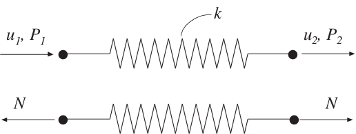
The spring element, shown below, can be used for the analysis of one dimensional spring systems and for a variety of analogous physical problems.

Quantities corresponding to the variables of the spring are listed in Table 1.
Problem type |
Spring stiffness |
Nodal displacement |
Element force |
Spring force |
|---|---|---|---|---|
Spring |
\(k\) |
\(u\) |
\(P\) |
\(N\) |
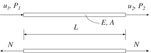
Bar |
\(\frac{EA}{L}\) |
\(u\) |
\(P\) |
\(N\) |
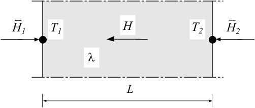
Thermal conduction |
\(\frac{\lambda A}{L}\) |
\(T\) |
\(\bar{H}\) |
\(H\) |
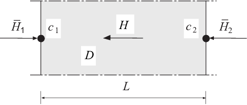
Diffusion |
\(\frac{D A}{L}\) |
\(c\) |
\(\bar{H}\) |
\(H\) |
Electrical circuit |
\(\frac{1}{R}\) |
\(U\) |
\(\bar{I}\) |
\(I\) |
Groundwater flow |
\(\frac{kA}{L}\) |
\(\phi\) |
\(\bar{H}\) |
\(H\) |
Pipe network |
\(\frac{\pi D^4}{128{\mu}L}\) |
\(p\) |
\(\bar{H}\) |
\(H\) |
Problem type |
Quantities |
Designations |
Description |
|---|---|---|---|
Spring |
|
\(k\), \(u\), \(P\), \(N\) |
spring stiffness, displacement, element force, spring force |
Bar |
|
\(L\), \(E\), \(A\), \(u\), \(P\), \(N\) |
length, modulus of elasticity, area of cross section, displacement, element force, normal force |
Thermal conduction |
|
\(L\), \(\lambda\), \(T\), \(\bar{H}\), \(H\) |
length, thermal conductivity, temperature, element heat flow, internal heat flow |
Diffusion |
|
\(L\), \(D\), \(c\), \(\bar{H}\), \(H\) |
length, diffusivity, nodal concentration, nodal mass flow, element mass flow |
Electrical circuit |
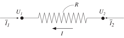
|
\(R\), \(U\), \(\bar{I}\), \(I\) |
resistance, potential, element current, internal current |
Groundwater flow |
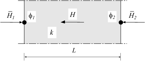
|
\(L\), \(k\), \(\phi\), \(\bar{H}\), \(H\) |
length, permeability, piezometric head, element water flow, internal water flow |
Pipe network (laminar flow) |
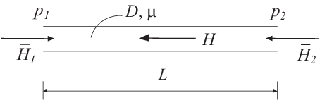
|
\(L\), \(D\), \(\mu\), \(p\), \(\bar{H}\), \(H\) |
length, pipe diameter, viscosity, pressure, element fluid flow, internal fluid flow |
The following functions are available for the spring element:
spring1e |
Compute element matrix |
spring1s |
Compute spring force |
spring1e
- Purpose:
Compute element stiffness matrix for a spring element.
- Syntax:
Ke = spring1e(ep)- Description:
spring1eprovides the element stiffness matrix \(\mathbf{K}^e\) for a spring element.The input variable
ep\(= [k]\)supplies the spring stiffness \(k\) or the analog quantity defined in Table Analogous quantities.
- Theory:
The element stiffness matrix \(\mathbf{K}^e\), stored in
Ke, is computed according to\[\begin{split}\mathbf{K}^e = \begin{bmatrix} k & -k \\ -k & k \end{bmatrix}\end{split}\]where \(k\) is defined by
ep.
spring1s
- Purpose:
Compute spring force in a spring element.

- Syntax:
es = spring1s(ep, ed)- Description:
spring1scomputes the spring force in the spring elementspring1e.The input variable
epis defined inspring1eand the element nodal displacementsedare obtained by the functionextract_ed.The output variable
es\(= [N]\)contains the spring force, or the analog quantity.
- Theory:
The spring force \(N\), or analog quantity, is computed according to
\[N = k \left(u_2 - u_1\right)\]
Bar element functions
Bar elements are available for one, two, and three dimensional analysis.
bar1e |
Compute element matrix |
bar1s |
Compute normal force |
bar1we |
Compute element matrix for element with elastic support |
bar1ws |
Compute normal force for element with elastic support |
bar2e |
Compute element matrix |
bar2s |
Compute normal force |
bar2ge |
Compute element matrix for geometric nonlinear element |
bar2gs |
Compute axial and normal forces for geometric nonlinear element |
bar3e |
Compute element matrix |
bar3s |
Compute normal force |
bar1e
- Purpose:
Compute element stiffness matrix for a one dimensional bar element.

- Syntax:
Ke = bar1e(ex, ep)
[Ke, fe] = bar1e(ex, ep, eq)
- Description:
bar1eprovides the element stiffness matrix \(\bar{\mathbf{K}}^e\) for a one dimensional bar element.The input variables
ex\(= [x_1 \;\; x_2]\) \(\qquad\)ep\(= [E \; A]\)supply the element nodal coordinates \(x_1\) and \(x_2\), the modulus of elasticity \(E\), and the cross section area \(A\).
The element load vector \(\bar{\mathbf{f}}_l^e\) can also be computed if a uniformly distributed load is applied to the element. The optional input variable
eq\(= [q_{\bar{x}}]\)contains the distributed load per unit length, \(q_{\bar{x}}\).

- Theory:
The element stiffness matrix \(\bar{\mathbf{K}}^e\), stored in
Ke, is computed according to\[\begin{split}\bar{\mathbf{K}}^e = \frac{D_{EA}}{L} \begin{bmatrix} 1 & -1 \\ -1 & 1 \end{bmatrix}\end{split}\]where the axial stiffness \(D_{EA}\) and the length \(L\) are given by
\[D_{EA} = EA; \quad L = x_2 - x_1\]The element load vector \(\bar{\mathbf{f}}_l^e\), stored in
fe, is computed according to\[\begin{split}\bar{\mathbf{f}}_l^e = \frac{q_{\bar{x}} L}{2} \begin{bmatrix} 1 \\ 1 \end{bmatrix}\end{split}\]
bar1s
- Purpose:
Compute normal force in a one dimensional bar element.

- Syntax:
es = bar1s(ex, ep, ed)
es = bar1s(ex, ep, ed, eq)
[es, edi] = bar1s(ex, ep, ed, eq, n)
[es, edi, eci] = bar1s(ex, ep, ed, eq, n)
- Description:
bar1scomputes the normal force in the one dimensional bar elementbar1e.The input variables
exandepare defined inbar1eand the element nodal displacements, stored ined, are obtained by the functionextract_ed. If distributed load is applied to the element, the variableeqmust be included.The number of evaluation points for normal force and displacement are determined by
n. Ifnis omitted, only the ends of the bar are evaluated.The output variables
es\(= \begin{bmatrix} N(0) \\ N(\bar{x}_2) \\ \vdots \\ N(\bar{x}_{n-1}) \\ N(L) \end{bmatrix}\) \(\qquad\)edi\(= \begin{bmatrix} u(0) \\ u(\bar{x}_2) \\ \vdots \\ u(\bar{x}_{n-1}) \\ u(L) \end{bmatrix}\) \(\qquad\)eci\(= \begin{bmatrix} 0 \\ \bar{x}_2 \\ \vdots \\ \bar{x}_{n-1} \\ L \end{bmatrix}\)contain the normal force, the displacement, and the evaluation points on the local \(\bar{x}\)-axis. \(L\) is the length of the bar element.
- Theory:
The nodal displacements in local coordinates are given by
\[\begin{split}\bar{\mathbf{a}}^e = \begin{bmatrix} \bar{u}_1 \\ \bar{u}_2 \end{bmatrix}\end{split}\]The transpose of \(\bar{\mathbf{a}}^e\) is stored in
ed.The displacement \(u(\bar{x})\) and the normal force \(N(\bar{x})\) are computed from
\[u(\bar{x}) = \mathbf{N} \bar{\mathbf{a}}^e + u_p(\bar{x})\]\[N(\bar{x}) = D_{EA} \mathbf{B} \bar{\mathbf{a}}^e + N_p(\bar{x})\]where
\[\mathbf{N} = \begin{bmatrix} 1 & \bar{x} \end{bmatrix} \mathbf{C}^{-1} = \begin{bmatrix} 1 - \frac{\bar{x}}{L} & \frac{\bar{x}}{L} \end{bmatrix}\]\[\mathbf{B} = \begin{bmatrix} 0 & 1 \end{bmatrix} \mathbf{C}^{-1} = \frac{1}{L} \begin{bmatrix} -1 & 1 \end{bmatrix}\]\[u_p(\bar{x}) = -\frac{q_{\bar{x}}}{D_{EA}} \left( \frac{\bar{x}^2}{2} - \frac{L\bar{x}}{2} \right)\]\[N_p(\bar{x}) = -q_{\bar{x}} \left( \bar{x} - \frac{L}{2} \right)\]in which \(D_{EA}\), \(L\), and \(q_{\bar{x}}\) are defined in
bar1eand\[\begin{split}\mathbf{C}^{-1} = \begin{bmatrix} 1 & 0 \\ -\frac{1}{L} & \frac{1}{L} \end{bmatrix}\end{split}\]
bar1we
- Purpose:
Compute element stiffness matrix for a one dimensional bar element with elastic support.

- Syntax:
Ke = bar1we(ex, ep)
[Ke, fe] = bar1we(ex, ep, eq)
- Description:
bar1weprovides the element stiffness matrix \(\bar{\mathbf{K}}^e\) for a one dimensional bar element with elastic support.The input variables
ex\(= [x_1\;\; x_2]\) \(\qquad\)ep\(= [E\; A\; k_{\bar{x}}]\)supply the element nodal coordinates \(x_1\) and \(x_2\), the modulus of elasticity \(E\), the cross section area \(A\) and the stiffness of the axial springs \(k_{\bar{x}}\).
The element load vector \(\bar{\mathbf{f}}_l^e\) can also be computed if a uniformly distributed load is applied to the element. The optional input variable
eq\(= [q_{\bar{x}}]\)contains the distributed load per unit length, \(q_{\bar{x}}\).
- Theory:
The element stiffness matrix \(\bar{\mathbf{K}}^e\), stored in
Ke, is computed according to\[\bar{\mathbf{K}}^e = \bar{\mathbf{K}}^e_0 + \bar{\mathbf{K}}^e_s\]where
\[\begin{split}\bar{\mathbf{K}}^e_0 = \frac{D_{EA}}{L} \begin{bmatrix} 1 & -1 \\ -1 & 1 \end{bmatrix}\end{split}\]\[\begin{split}\bar{\mathbf{K}}^e_s = k_{\bar{x}} L \begin{bmatrix} \frac{1}{3} & \frac{1}{6} \\ \frac{1}{6} & \frac{1}{3} \end{bmatrix}\end{split}\]where the axial stiffness \(D_{EA}\) and the length \(L\) are given by
\[D_{EA} = EA; \qquad L = x_2 - x_1\]The element load vector \(\bar{\mathbf{f}}_l^e\), stored in
fe, is computed according to\[\begin{split}\bar{\mathbf{f}}_l^e = \frac{q_{\bar{x}} L}{2} \begin{bmatrix} 1 \\ 1 \end{bmatrix}\end{split}\]
bar1ws
- Purpose:
Compute normal force in a one dimensional bar element with elastic support.
- Syntax:
es = bar1ws(ex, ep, ed)
es = bar1ws(ex, ep, ed, eq)
[es, edi] = bar1ws(ex, ep, ed, eq, n)
[es, edi, eci] = bar1ws(ex, ep, ed, eq, n)
- Description:
bar1wscomputes the normal force in the one dimensional bar elementbar1we.The input variables
exandepare defined inbar1weand the element nodal displacements, stored ined, are obtained by the functionextract_ed. If distributed load is applied to the element, the variableeqmust be included.The number of evaluation points for normal force and displacement are determined by
n. Ifnis omitted, only the ends of the bar are evaluated.The output variables are:
es\(= \begin{bmatrix} N(0) \\ N(\bar{x}_2) \\ \vdots \\ N(\bar{x}_{n-1}) \\ N(L) \end{bmatrix}\) \(\qquad\)edi\(= \begin{bmatrix} u(0) \\ u(\bar{x}_2) \\ \vdots \\ u(\bar{x}_{n-1}) \\ u(L) \end{bmatrix}\) \(\qquad\)eci\(= \begin{bmatrix} 0 \\ \bar{x}_2 \\ \vdots \\ \bar{x}_{n-1} \\ L \end{bmatrix}\)These contain the normal force, the displacement, and the evaluation points on the local \(\bar{x}\)-axis. \(L\) is the length of the bar element.
- Theory:
The nodal displacements in local coordinates are given by
\[\begin{split}\bar{\mathbf{a}}^e = \begin{bmatrix} \bar{u}_1 \\ \bar{u}_2 \end{bmatrix}\end{split}\]The transpose of \(\bar{\mathbf{a}}^e\) is stored in
ed.The displacement \(u(\bar{x})\) and the normal force \(N(\bar{x})\) are computed from
\[u(\bar{x}) = \mathbf{N} \bar{\mathbf{a}}^e + u_p(\bar{x})\]\[N(\bar{x}) = D_{EA} \mathbf{B} \bar{\mathbf{a}}^e + N_p(\bar{x})\]where
\[\mathbf{N} = \begin{bmatrix} 1 & \bar{x} \end{bmatrix} \mathbf{C}^{-1} = \begin{bmatrix} 1 - \frac{\bar{x}}{L} & \frac{\bar{x}}{L} \end{bmatrix}\]\[\mathbf{B} = \begin{bmatrix} 0 & 1 \end{bmatrix} \mathbf{C}^{-1} = \frac{1}{L} \begin{bmatrix} -1 & 1 \end{bmatrix}\]\[u_p(\bar{x}) = \frac{k_{\bar{x}}}{D_{EA}} \left[ \frac{\bar{x}^2 - L\bar{x}}{2} \quad \frac{\bar{x}^3 - L^2\bar{x}}{6} \right] \mathbf{C}^{-1} \bar{\mathbf{a}}^e - \frac{q_{\bar{x}}}{D_{EA}} \left( \frac{\bar{x}^2}{2} - \frac{L\bar{x}}{2} \right)\]\[N_p(\bar{x}) = k_{\bar{x}} \left[ \frac{2\bar{x} - L}{2} \quad \frac{3\bar{x}^2 - L^2}{6} \right] \mathbf{C}^{-1} \bar{\mathbf{a}}^e - q_{\bar{x}} \left( \bar{x} - \frac{L}{2} \right)\]in which \(D_{EA}\), \(L\), \(k_{\bar{x}}\) and \(q_{\bar{x}}\) are defined in
bar1weand\[\begin{split}\mathbf{C}^{-1} = \begin{bmatrix} 1 & 0 \\ -\frac{1}{L} & \frac{1}{L} \end{bmatrix}\end{split}\]
bar2e
- Purpose:
Compute element stiffness matrix for a two dimensional bar element.

- Syntax:
Ke = bar2e(ex, ey, ep)
[Ke, fe] = bar2e(ex, ey, ep, eq)
- Description:
bar2eprovides the global element stiffness matrix \({\mathbf{K}}^e\) for a two dimensional bar element.The input variables
ex\(= [x_1 \;\; x_2]\) \(\qquad\)ey\(= [y_1 \;\; y_2]\) \(\qquad\)ep\(= [E \; A]\)supply the element nodal coordinates \(x_1\), \(y_1\), \(x_2\), and \(y_2\), the modulus of elasticity \(E\), and the cross section area \(A\).
The element load vector \({\mathbf{f}}_l^e\) can also be computed if a uniformly distributed load is applied to the element. The optional input variable
eq\(= [q_{\bar{x}}]\)contains the distributed load per unit length, \(q_{\bar{x}}\).

- Theory:
The element stiffness matrix \(\mathbf{K}^e\), stored in
Ke, is computed according to\[\mathbf{K}^e = \mathbf{G}^T \; \bar{\mathbf{K}}^e \; \mathbf{G}\]where
\[\begin{split}\bar{\mathbf{K}}^e = \frac{D_{EA}}{L} \begin{bmatrix} 1 & -1 \\ -1 & 1 \end{bmatrix} \qquad \mathbf{G} = \begin{bmatrix} n_{x\bar{x}} & n_{y\bar{x}} & 0 & 0 \\ 0 & 0 & n_{x\bar{x}} & n_{y\bar{x}} \end{bmatrix}\end{split}\]where the axial stiffness \(D_{EA}\) and the length \(L\) are given by
\[D_{EA} = EA; \qquad L = \sqrt{(x_2 - x_1)^2 + (y_2 - y_1)^2}\]and the transformation matrix \(\mathbf{G}\) contains the direction cosines
\[n_{x\bar{x}} = \frac{x_2 - x_1}{L} \qquad n_{y\bar{x}} = \frac{y_2 - y_1}{L}\]The element load vector \(\mathbf{f}_l^e\), stored in
fe, is computed according to\[\mathbf{f}_l^e = \mathbf{G}^T \; \bar{\mathbf{f}}_l^e\]where
\[\begin{split}\bar{\mathbf{f}}_l^e = \frac{q_{\bar{x}} L}{2} \begin{bmatrix} 1 \\ 1 \end{bmatrix}\end{split}\]
bar2s
- Purpose:
Compute normal force in a two dimensional bar element.

- Syntax:
es = bar2s(ex, ey, ep, ed)
es = bar2s(ex, ey, ep, ed, eq)
[es, edi] = bar2s(ex, ey, ep, ed, eq, n)
[es, edi, eci] = bar2s(ex, ey, ep, ed, eq, n)
- Description:
bar2scomputes the normal force in the two dimensional bar elementbar2e.The input variables
ex,ey, andepare defined inbar2eand the element nodal displacements, stored ined, are obtained by the functionextract_ed. If distributed loads are applied to the element, the variableeqmust be included. The number of evaluation points for section forces and displacements are determined byn. Ifnis omitted, only the ends of the bar are evaluated.The output variables
es\(= \begin{bmatrix} N(0) \\ N(\bar{x}_2) \\ \vdots \\ N(\bar{x}_{n-1}) \\ N(L) \end{bmatrix}\) \(\qquad\)edi\(= \begin{bmatrix} u(0) \\ u(\bar{x}_2) \\ \vdots \\ u(\bar{x}_{n-1}) \\ u(L) \end{bmatrix}\) \(\qquad\)eci\(= \begin{bmatrix} 0 \\ \bar{x}_2 \\ \vdots \\ \bar{x}_{n-1} \\ L \end{bmatrix}\)contain the normal force, the displacement, and the evaluation points on the local \(\bar{x}\)-axis. \(L\) is the length of the bar element.
- Theory:
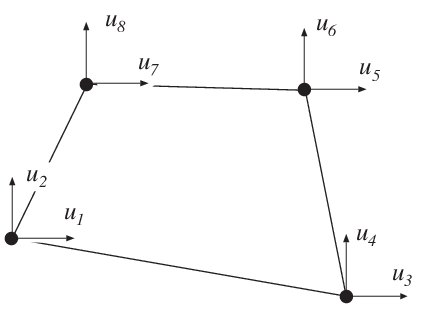
The nodal displacements in global coordinates
\[\mathbf{a}^e = \begin{bmatrix} u_1 & u_2 & u_3 & u_4 \end{bmatrix}^T\]are also shown in
bar2e. The transpose of \(\mathbf{a}^e\) is stored ined.The nodal displacements in local coordinates are given by
\[\bar{\mathbf{a}}^e = \mathbf{G} \mathbf{a}^e\]where the transformation matrix \(\mathbf{G}\) is defined in
bar2e.The displacement \(u(\bar{x})\) and the normal force \(N(\bar{x})\) are computed from
\[u(\bar{x}) = \mathbf{N} \bar{\mathbf{a}}^e + u_p(\bar{x})\]\[N(\bar{x}) = D_{EA} \mathbf{B} \bar{\mathbf{a}}^e + N_p(\bar{x})\]where
\[\mathbf{N} = \begin{bmatrix} 1 & \bar{x} \end{bmatrix} \mathbf{C}^{-1} = \begin{bmatrix} 1-\frac{\bar{x}}{L} & \frac{\bar{x}}{L} \end{bmatrix}\]\[\mathbf{B} = \begin{bmatrix} 0 & 1 \end{bmatrix} \mathbf{C}^{-1} = \frac{1}{L} \begin{bmatrix} -1 & 1 \end{bmatrix}\]\[u_p(\bar{x}) = -\frac{q_{\bar{x}}}{D_{EA}}\left(\frac{\bar{x}^2}{2}-\frac{L\bar{x}}{2}\right)\]\[N_p(\bar{x}) = -q_{\bar{x}}\left(\bar{x}-\frac{L}{2}\right)\]where \(D_{EA}\), \(L\), \(q_{\bar{x}}\) are defined in
bar2eand\[\begin{split}\mathbf{C}^{-1} = \begin{bmatrix} 1 & 0 \\ -\frac{1}{L} & \frac{1}{L} \end{bmatrix}\end{split}\]
bar2ge
- Purpose:
Compute element stiffness matrix for a two dimensional bar element with geometric nonlinearity.

- Syntax:
Ke = bar2ge(ex, ey, ep, Qx)
- Description:
bar2geprovides the global element stiffness matrix \({\mathbf{K}}^e\) for a two dimensional bar element with geometric nonlinearity.The input variables
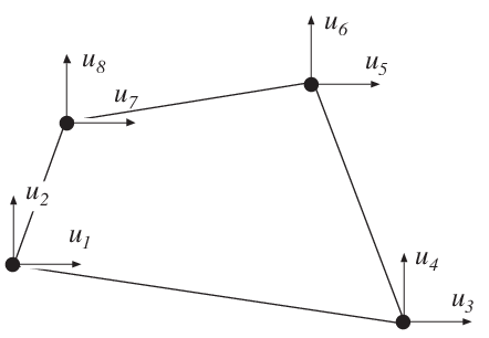
ex\(= [x_1 \;\; x_2]\) \(\qquad\)ey\(= [y_1 \;\; y_2]\) \(\qquad\)ep\(= [E \; A]\)supply the element nodal coordinates \(x_1\), \(y_1\), \(x_2\), and \(y_2\), the modulus of elasticity \(E\), and the cross section area \(A\).
The input variable
Qx\(= [Q_{\bar{x}}]\)contains the value of the axial force, which is positive in tension.
- Theory:
The global element stiffness matrix \(\mathbf{K}^e\), stored in
Ke, is computed according to\[\mathbf{K}^e = \mathbf{G}^T\,\bar{\mathbf{K}}^e\,\mathbf{G}\]where \(\bar{\mathbf{K}}^e\) is given by
\[\bar{\mathbf{K}}^e = \bar{\mathbf{K}}^e_0 + \bar{\mathbf{K}}^e_{\sigma}\]with
\[\begin{split}\bar{\mathbf{K}}^e_0 = \frac{D_{EA}}{L} \begin{bmatrix} 1 & 0 & -1 & 0 \\ 0 & 0 & 0 & 0 \\ -1 & 0 & 1 & 0 \\ 0 & 0 & 0 & 0 \end{bmatrix}\end{split}\]\[\begin{split}\bar{\mathbf{K}}^e_{\sigma} = \frac{Q_{\bar{x}}}{L} \begin{bmatrix} 0 & 0 & 0 & 0 \\ 0 & 1 & 0 & -1 \\ 0 & 0 & 0 & 0 \\ 0 & -1 & 0 & 1 \end{bmatrix}\end{split}\]\[\begin{split}\mathbf{G} = \begin{bmatrix} n_{x\bar{x}} & n_{y\bar{x}} & 0 & 0 \\ n_{x\bar{y}} & n_{y\bar{y}} & 0 & 0 \\ 0 & 0 & n_{x\bar{x}} & n_{y\bar{x}} \\ 0 & 0 & n_{x\bar{y}} & n_{y\bar{y}} \end{bmatrix}\end{split}\]where the axial stiffness \(D_{EA}\) and the length \(L\) are given by
\[D_{EA} = EA \qquad L = \sqrt{(x_2 - x_1)^2 + (y_2 - y_1)^2}\]and the transformation matrix \(\mathbf{G}\) contains the direction cosines
\[n_{x\bar{x}} = n_{y\bar{y}} = \frac{x_2 - x_1}{L} \qquad n_{y\bar{x}} = -n_{x\bar{y}} = \frac{y_2 - y_1}{L}\]
bar2gs
- Purpose:
Compute normal force in a two dimensional bar element with geometric nonlinearity.
- Syntax:
[es, Qx] = bar2gs(ex, ey, ep, ed)
[es, Qx, edi] = bar2gs(ex, ey, ep, ed, n)
[es, Qx, edi, eci] = bar2gs(ex, ey, ep, ed, n)
- Description:
bar2gscomputes the normal force, axial force and displacements in the two dimensional bar elementbar2ge.The input variables
ex,ey, andepare defined inbar2geand the element nodal displacements, stored ined, are obtained by the functionextract_ed. The number of evaluation points for section forces and displacements are determined byn. Ifnis omitted, only the ends of the bar are evaluated.The output variable
Qxcontains the axial force \(Q_{\bar{x}}\) and the output variableses\(= \begin{bmatrix} N(0) \\ N(\bar{x}_2) \\ \vdots \\ N(\bar{x}_{n-1}) \\ N(L) \end{bmatrix}\) \(\qquad\)edi\(= \begin{bmatrix} u(0) \\ u(\bar{x}_2) \\ \vdots \\ u(\bar{x}_{n-1}) \\ u(L) \end{bmatrix}\) \(\qquad\)eci\(= \begin{bmatrix} 0 \\ \bar{x}_2 \\ \vdots \\ \bar{x}_{n-1} \\ L \end{bmatrix}\)contain the normal force, the displacement, and the evaluation points on the local \(\bar{x}\)-axis. \(L\) is the length of the bar element.
- Theory:
The nodal displacements in global coordinates are given by
\[\mathbf{a}^e = \left[\; u_1\;\; u_2\;\; u_3\;\; u_4 \;\right]^T\]The transpose of \(\mathbf{a}^e\) is stored in
ed. The nodal displacements in local coordinates are given by\[\bar{\mathbf{a}}^e = \mathbf{G} \mathbf{a}^e\]where the transformation matrix \(\mathbf{G}\) is defined in
bar2ge. The displacements associated with bar action are determined as\[\begin{split}\bar{\mathbf{a}}^e_{\text{bar}} = \left[ \begin{array}{r} \bar{u}_1 \\ \bar{u}_3 \end{array}\right]\end{split}\]The displacement \(u(\bar{x})\) and the normal force \(N(\bar{x})\) are computed from
\[u(\bar{x}) = {\mathbf{N}} \bar{\mathbf{a}}^e_{\text{bar}}\]\[N(\bar{x}) = D_{EA} \mathbf{B} \bar{\mathbf{a}}^e_{\text{bar}}\]where
\[\mathbf{N} = \left[\begin{array}{rr} 1 & \bar{x} \end{array}\right] \mathbf{C}^{-1} = \left[\begin{array}{rr} 1-\frac{\bar{x}}{L} & \frac{\bar{x}}{L} \end{array}\right]\]\[\mathbf{B} = \left[\begin{array}{rr} 0 & 1 \end{array}\right] \mathbf{C}^{-1} = \frac{1}{L}\left[\begin{array}{rr} -1 & 1 \end{array}\right]\]where \(D_{EA}\) and \(L\) are defined in
bar2geand\[\begin{split}\mathbf{C}^{-1} = \left[ \begin{array}{rr} 1 & 0 \\ -\frac{1}{L} & \frac{1}{L} \end{array}\right]\end{split}\]An updated value of the axial force is computed as
\[Q_{\bar{x}} = N(0)\]
bar3e
- Purpose:
Compute element stiffness matrix for a three dimensional bar element.

- Syntax:
Ke = bar3e(ex, ey, ez, ep)
[Ke, fe] = bar3e(ex, ey, ez, ep, eq)
- Description:
bar3eprovides the global element stiffness matrix \({\mathbf{K}}^e\) for a three dimensional bar element.The input variables
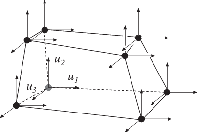
ex\(= [x_1 \;\; x_2]\) \(\qquad\)ey\(= [y_1 \;\; y_2]\) \(\qquad\)ez\(= [z_1 \;\; z_2]\) \(\qquad\)ep\(= [E \; A]\)supply the element nodal coordinates \(x_1\), \(y_1\), \(z_1\), \(x_2\), \(y_2\), and \(z_2\), the modulus of elasticity \(E\), and the cross section area \(A\).
The element load vector
fecan also be computed if a uniformly distributed axial load is applied to the element. The optional input variableeq\(= [q_{\bar{x}}]\)contains the distributed load per unit length, \(q_{\bar{x}}\).
- Theory:
The element stiffness matrix \(\mathbf{K}^e\), stored in
Ke, is computed according to\[\mathbf{K}^e = \mathbf{G}^T \; \bar{\mathbf{K}}^e \; \mathbf{G}\]where
\[\begin{split}\bar{\mathbf{K}}^e = \frac{D_{EA}}{L} \begin{bmatrix} 1 & -1 \\ -1 & 1 \end{bmatrix} \qquad \mathbf{G} = \begin{bmatrix} n_{x\bar{x}} & n_{y\bar{x}} & n_{z\bar{x}} & 0 & 0 & 0 \\ 0 & 0 & 0 & n_{x\bar{x}} & n_{y\bar{x}} & n_{z\bar{x}} \end{bmatrix}\end{split}\]where the axial stiffness \(D_{EA}\) and the length \(L\) are given by
\[D_{EA} = EA \qquad L = \sqrt{(x_2 - x_1)^2 + (y_2 - y_1)^2 + (z_2 - z_1)^2}\]and the transformation matrix \(\mathbf{G}\) contains the direction cosines
\[n_{x\bar{x}} = \frac{x_2 - x_1}{L} \qquad n_{y\bar{x}} = \frac{y_2 - y_1}{L} \qquad n_{z\bar{x}} = \frac{z_2 - z_1}{L}\]The element load vector \(\mathbf{f}_l^e\), stored in
fe, is computed according to\[\mathbf{f}_l^e = \mathbf{G}^T \; \bar{\mathbf{f}}_l^e\]where
\[\begin{split}\bar{\mathbf{f}}_l^e = \frac{q_{\bar{x}} L}{2} \begin{bmatrix} 1 \\ 1 \end{bmatrix}\end{split}\]
bar3s
- Purpose:
Compute normal force in a three dimensional bar element.

- Syntax:
es = bar3s(ex, ey, ez, ep, ed)
es = bar3s(ex, ey, ez, ep, ed, eq)
[es, edi] = bar3s(ex, ey, ez, ep, ed, eq, n)
[es, edi, eci] = bar3s(ex, ey, ez, ep, ed, eq, n)
- Description:
bar3scomputes the normal force in the three dimensional bar elementbar3e.The input variables
ex,ey, andepare defined inbar3eand the element nodal displacements, stored ined, are obtained by the functionextract_ed. The number of evaluation points for section forces and displacements are determined byn. Ifnis omitted, only the ends of the bar are evaluated.The output variables
es\(= \begin{bmatrix} N(0) \\ N(\bar{x}_2) \\ \vdots \\ N(\bar{x}_{n-1}) \\ N(L) \end{bmatrix}\) \(\qquad\)edi\(= \begin{bmatrix} u(0) \\ u(\bar{x}_2) \\ \vdots \\ u(\bar{x}_{n-1}) \\ u(L) \end{bmatrix}\) \(\qquad\)eci\(= \begin{bmatrix} 0 \\ \bar{x}_2 \\ \vdots \\ \bar{x}_{n-1} \\ L \end{bmatrix}\) \(\qquad\)contain the normal force, the displacement, and the evaluation points on the local \(\bar{x}\)-axis. \(L\) is the length of the bar element.
- Theory:
The nodal displacements in global coordinates are given by
\[\mathbf{a}^e = \begin{bmatrix} u_1 & u_2 & u_3 & u_4 & u_5 & u_6 \end{bmatrix}^T\]The transpose of \(\mathbf{a}^e\) is stored in
ed.The nodal displacements in local coordinates are given by
\[\bar{\mathbf{a}}^e = \mathbf{G} \mathbf{a}^e\]where the transformation matrix \(\mathbf{G}\) is defined in
bar3e.The displacement \(u(\bar{x})\) and the normal force \(N(\bar{x})\) are computed from
\[u(\bar{x}) = \mathbf{N} \bar{\mathbf{a}}^e + u_p(\bar{x})\]\[N(\bar{x}) = D_{EA} \mathbf{B} \bar{\mathbf{a}}^e + N_p(\bar{x})\]where
\[\mathbf{N} = \begin{bmatrix} 1 & \bar{x} \end{bmatrix} \mathbf{C}^{-1} = \begin{bmatrix} 1-\frac{\bar{x}}{L} & \frac{\bar{x}}{L} \end{bmatrix}\]\[\mathbf{B} = \begin{bmatrix} 0 & 1 \end{bmatrix} \mathbf{C}^{-1} = \frac{1}{L} \begin{bmatrix} -1 & 1 \end{bmatrix}\]\[u_p(\bar{x}) = -\frac{q_{\bar{x}}}{D_{EA}} \left( \frac{\bar{x}^2}{2} - \frac{L\bar{x}}{2} \right)\]\[N_p(\bar{x}) = -q_{\bar{x}} \left( \bar{x} - \frac{L}{2} \right)\]where \(D_{EA}\), \(L\), \(q_{\bar{x}}\) are defined in
bar3eand\[\begin{split}\mathbf{C}^{-1} = \begin{bmatrix} 1 & 0 \\ -\frac{1}{L} & \frac{1}{L} \end{bmatrix}\end{split}\]
Heat Flow Elements
Heat flow elements are available for one, two, and three dimensional analysis.
For one dimensional heat flow the spring element spring1 is used.
A variety of important physical phenomena are described by the same differential equation as the heat flow problem. The heat flow element is thus applicable in modelling different physical applications. Table below shows the relation between the primary variable a, the constitutive matrix D, and the load vector f_l for a chosen set of two dimensional physical problems.
Problem type |
a |
D |
f_l |
Designation |
|---|---|---|---|---|
Heat flow |
\(T\) |
\(\lambda_x\), \(\lambda_y\) |
\(Q\) |
|
Groundwater flow |
\(\phi\) |
\(k_x\), \(k_y\) |
\(Q\) |
|
St. Venant torsion |
\(\phi\) |
\(1/G_{zy}\), \(1/G_{zx}\) |
\(2\Theta\) |
|
|
|
|
|
flw2te |
Compute element matrices for a triangular element |
flw2ts |
Compute temperature gradients and flux |
flw2qe |
Compute element matrices for a quadrilateral element |
flw2qs |
Compute temperature gradients and flux |
flw2i4e |
Compute element matrices, 4 node isoparametric element |
flw2i4s |
Compute temperature gradients and flux |
flw2i8e |
Compute element matrices, 8 node isoparametric element |
flw2i8s |
Compute temperature gradients and flux |
flw3i8e |
Compute element matrices, 8 node isoparametric element |
flw3i8s |
Compute temperature gradients and flux |
flw2te
- Purpose:
Compute element stiffness matrix for a triangular heat flow element.

- Syntax:
Ke = flw2te(ex, ey, ep, D) [Ke, fe] = flw2te(ex, ey, ep, D, eq)- Description:
flw2teprovides the element stiffness (conductivity) matrixKeand the element load vectorfefor a triangular heat flow element.The element nodal coordinates \(x_1\), \(y_1\), \(x_2\) etc, are supplied to the function by
exandey, the element thickness \(t\) is supplied byepand the thermal conductivities (or corresponding quantities) \(k_{xx}\), \(k_{xy}\) etc are supplied byD.\[\begin{split}\begin{array}{l} \mathbf{ex} = [\, x_1 \;\; x_2 \;\; x_3\,] \\ \mathbf{ey} = [\, y_1 \;\; y_2 \;\; y_3\,] \end{array} \qquad \mathbf{ep} = [\, t \,] \qquad \mathbf{D} = \begin{bmatrix} k_{xx} & k_{xy} \\ k_{yx} & k_{yy} \end{bmatrix}\end{split}\]If the scalar variable
eqis given in the function, the element load vector \(\mathbf{fe}\) is computed, using\[\mathbf{eq} = [\, Q \,]\]where \(Q\) is the heat supply per unit volume.
- Theory:
The element stiffness matrix \(\mathbf{K}^e\) and the element load vector \(\mathbf{f}_l^e\), stored in
Keandfe, respectively, are computed according to\[\mathbf{K}^e = (\mathbf{C}^{-1})^T \int_A \bar{\mathbf{B}}^T \mathbf{D} \bar{\mathbf{B}}\, t\, dA\, \mathbf{C}^{-1}\]\[\mathbf{f}_l^e = (\mathbf{C}^{-1})^T \int_A \bar{\mathbf{N}}^T Q\, t\, dA\]with the constitutive matrix \(\mathbf{D}\) defined by
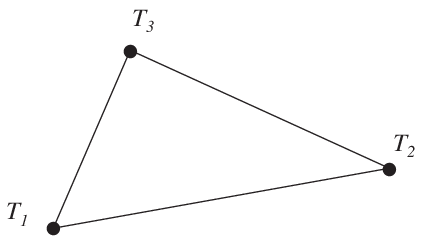
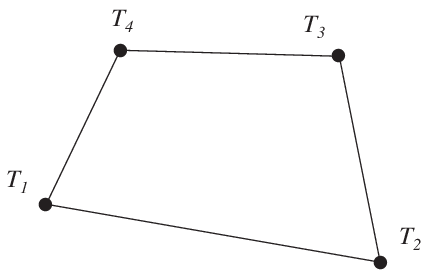
D.The evaluation of the integrals for the triangular element is based on the linear temperature approximation \(T(x, y)\) and is expressed in terms of the nodal variables \(T_1\), \(T_2\) and \(T_3\) as
\[T(x, y) = \mathbf{N}^e \mathbf{a}^e = \bar{\mathbf{N}}\, \mathbf{C}^{-1} \mathbf{a}^e\]where
\[\begin{split}\bar{\mathbf{N}} = [\, 1 \;\; x \;\; y\,] \qquad \mathbf{C} = \begin{bmatrix} 1 & x_1 & y_1 \\ 1 & x_2 & y_2 \\ 1 & x_3 & y_3 \end{bmatrix} \qquad \mathbf{a}^e = \begin{bmatrix} T_1 \\ T_2 \\ T_3 \end{bmatrix}\end{split}\]and hence it follows that
\[\begin{split}\bar{\mathbf{B}} = \nabla \bar{\mathbf{N}} = \begin{bmatrix} 0 & 1 & 0 \\ 0 & 0 & 1 \end{bmatrix} \qquad \nabla = \begin{bmatrix} \dfrac{\partial}{\partial x} \\ \dfrac{\partial}{\partial y} \end{bmatrix}\end{split}\]Evaluation of the integrals for the triangular element yields
\[\mathbf{K}^e = (\mathbf{C}^{-1})^T \bar{\mathbf{B}}^T \mathbf{D} \bar{\mathbf{B}} \mathbf{C}^{-1} t A\]\[\begin{split}\mathbf{f}_l^e = \frac{Q A t}{3} \begin{bmatrix} 1 \\ 1 \\ 1 \end{bmatrix}\end{split}\]where the element area \(A\) is determined as
\[A = \frac{1}{2} \det \mathbf{C}\]
flw2ts
- Purpose:
Compute heat flux and temperature gradients in a triangular heat flow element.
- Syntax:
[es, et] = flw2ts(ex, ey, D, ed)- Description:
flw2tscomputes the heat flux vectoresand the temperature gradientet(or corresponding quantities) in a triangular heat flow element.The input variables
ex,eyand the matrixDare defined inflw2te. The vectoredcontains the nodal temperatures \(\mathbf{a}^e\) of the element and is obtained by the functionextractas\[\mathbf{ed} = (\mathbf{a}^e)^T = [\;T_1\;\; T_2\;\; T_3\;]\]The output variables
\[\mathbf{es} = \mathbf{q}^T = \left[\; q_x \; q_y \;\right]\]\[\mathbf{et} = (\nabla T)^T = \left[\begin{array}{l} \frac{\partial T}{\partial x}\;\;\frac{\partial T}{\partial y} \end{array} \right]\]contain the components of the heat flux and the temperature gradient computed in the directions of the coordinate axis.
- Theory:
The temperature gradient and the heat flux are computed according to
\[\nabla T = \bar{\mathbf{B}}\;\mathbf{C}^{-1}\;\mathbf{a}^e\]\[\mathbf{q} = - \mathbf{D} \nabla T\]where the matrices \(\mathbf{D}\), \(\bar{\mathbf{B}}\), and \(\mathbf{C}\) are described in
flw2te. Note that both the temperature gradient and the heat flux are constant in the element.
flw2qe
- Purpose:
Compute element stiffness matrix for a quadrilateral heat flow element.

- Syntax:
Ke = flw2qe(ex, ey, ep, D) [Ke, fe] = flw2qe(ex, ey, ep, D, eq)- Description:
flw2qeprovides the element stiffness (conductivity) matrixKeand the element load vectorfefor a quadrilateral heat flow element.The element nodal coordinates \(x_1\), \(y_1\), \(x_2\) etc, are supplied to the function by
exandey, the element thickness \(t\) is supplied byepand the thermal conductivities (or corresponding quantities) \(k_{xx}\), \(k_{xy}\) etc are supplied byD.\[\begin{split}\begin{array}{l} \mathbf{ex} = [\, x_1 \;\; x_2 \;\; x_3 \;\; x_4 \,] \\ \mathbf{ey} = [\, y_1 \;\; y_2 \;\; y_3 \;\; y_4 \,] \end{array} \qquad \mathbf{ep} = \left[\, t \,\right] \qquad \mathbf{D} = \left[ \begin{array}{cc} k_{xx} & k_{xy} \\ k_{yx} & k_{yy} \end{array} \right]\end{split}\]If the scalar variable
eqis given in the function, the element load vector \(\mathbf{fe}\) is computed, using\[\mathbf{eq} = \left[\, Q \,\right]\]where \(Q\) is the heat supply per unit volume.
- Theory:
In computing the element matrices, a fifth degree of freedom is introduced. The location of this extra degree of freedom is defined by the mean value of the coordinates in the corner points. Four sets of element matrices are calculated using
flw2te. These matrices are then assembled and the fifth degree of freedom is eliminated by static condensation.
flw2qs
- Purpose:
Compute heat flux and temperature gradients in a quadrilateral heat flow element.
- Syntax:
[es, et] = flw2qs(ex, ey, ep, D, ed) [es, et] = flw2qs(ex, ey, ep, D, ed, eq)- Description:
flw2qscomputes the heat flux vectoresand the temperature gradientet(or corresponding quantities) in a quadrilateral heat flow element.The input variables
ex,ey,eqand the matrixDare defined inflw2qe. The vectoredcontains the nodal temperatures \(\mathbf{a}^e\) of the element and is obtained by the functionextractas\[\mathbf{ed} = (\mathbf{a}^e)^T = [\;T_1\;\; T_2\;\; T_3\;\; T_4\;]\]The output variables
\[\mathbf{es} = \mathbf{q}^T = \left[\; q_x \; q_y \;\right]\]\[\mathbf{et} = (\nabla T)^T = \left[\begin{array}{l} \frac{\partial T}{\partial x}\;\;\frac{\partial T}{\partial y} \end{array} \right]\]contain the components of the heat flux and the temperature gradient computed in the directions of the coordinate axis.
- Theory:
By assembling four triangular elements as described in
flw2tea system of equations containing 5 degrees of freedom is obtained. From this system of equations the unknown temperature at the center of the element is computed. Then according to the description inflw2tsthe temperature gradient and the heat flux in each of the four triangular elements are produced. Finally the temperature gradient and the heat flux of the quadrilateral element are computed as area weighted mean values from the values of the four triangular elements. If heat is supplied to the element, the element load vectoreqis needed for the calculations.Note
If the input variables are given for a number of identical (
nie) elements, i.e.Ex,Ey, andEdare matrices, then the output variables are defined as\[\begin{split}\mathrm{Es} = \left[ \begin{array}{cc} q^1_x & q^1_y \\ q^2_x & q^2_y \\ \vdots & \vdots \\ q^{nie}_x & q^{nie}_y \end{array} \right] \qquad \mathrm{Et} = \left[ \begin{array}{cc} \frac{\partial T}{\partial x}^1 & \frac{\partial T}{\partial y}^1 \\ \frac{\partial T}{\partial x}^2 & \frac{\partial T}{\partial y}^2 \\ \vdots & \vdots \\ \frac{\partial T}{\partial x}^{nie} & \frac{\partial T}{\partial y}^{nie} \end{array} \right]\end{split}\]where \(\mathbf{q}^i\) and \(\nabla T^i\) are computed from the nodal values located in column
iofEd.
flw2i4e
- Purpose:
Compute element stiffness matrix for a 4 node isoparametric heat flow element.

- Syntax:
Ke = flw2i4e(ex, ey, ep, D) [Ke, fe] = flw2i4e(ex, ey, ep, D, eq)- Description:
flw2i4eprovides the element stiffness (conductivity) matrixKeand the element load vectorfefor a 4 node isoparametric heat flow element.The element nodal coordinates \(x_1\), \(y_1\), \(x_2\) etc, are supplied to the function by
exandey. The element thickness \(t\) and the number of Gauss points \(n\) (\(n \times n\) integration points, \(n=1,2,3\)) are supplied to the function byepand the thermal conductivities (or corresponding quantities) \(k_{xx}\), \(k_{xy}\) etc are supplied byD.\[\begin{split}\begin{array}{l} \mathbf{ex} = [\, x_1 \;\; x_2 \;\; x_3 \;\; x_4 \,] \\ \mathbf{ey} = [\, y_1 \;\; y_2 \;\; y_3 \;\; y_4 \,] \end{array} \qquad \mathbf{ep} = [\, t \;\; n \,] \qquad \mathbf{D} = \begin{bmatrix} k_{xx} & k_{xy} \\ k_{yx} & k_{yy} \end{bmatrix}\end{split}\]If the scalar variable
eqis given in the function, the element load vector \(fe\) is computed, using\[\mathbf{eq} = [\, Q \,]\]where \(Q\) is the heat supply per unit volume.
- Theory:
The element stiffness matrix \(\mathbf{K}^e\) and the element load vector \(\mathbf{f}_l^e\), stored in
Keandfe, respectively, are computed according to\[\mathbf{K}^e = \int_A \mathbf{B}^{eT} \mathbf{D} \mathbf{B}^e t\, dA\]\[\mathbf{f}_l^e = \int_A \mathbf{N}^{eT} Q t\, dA\]with the constitutive matrix \(\mathbf{D}\) defined by
D.The evaluation of the integrals for the isoparametric 4 node element is based on a temperature approximation \(T(\xi, \eta)\), expressed in a local coordinate system in terms of the nodal variables \(T_1\), \(T_2\), \(T_3\) and \(T_4\) as
\[T(\xi, \eta) = \mathbf{N}^e \mathbf{a}^e\]where
\[\mathbf{N}^e = [\, N_1^e \;\; N_2^e \;\; N_3^e \;\; N_4^e \,] \qquad \mathbf{a}^e = [\, T_1 \;\; T_2 \;\; T_3 \;\; T_4 \,]^T\]The element shape functions are given by
\[\begin{split}N_1^e = \frac{1}{4}(1-\xi)(1-\eta) \qquad N_2^e = \frac{1}{4}(1+\xi)(1-\eta) \\ N_3^e = \frac{1}{4}(1+\xi)(1+\eta) \qquad N_4^e = \frac{1}{4}(1-\xi)(1+\eta)\end{split}\]The \(\mathbf{B}^e\)-matrix is given by
\[\begin{split}\mathbf{B}^e = \nabla \mathbf{N}^e = \begin{bmatrix} \frac{\partial}{\partial x} \\ \frac{\partial}{\partial y} \end{bmatrix} \mathbf{N}^e = (\mathbf{J}^T)^{-1} \begin{bmatrix} \frac{\partial}{\partial \xi} \\ \frac{\partial}{\partial \eta} \end{bmatrix} \mathbf{N}^e\end{split}\]where \(\mathbf{J}\) is the Jacobian matrix
\[\begin{split}\mathbf{J} = \begin{bmatrix} \frac{\partial x}{\partial \xi} & \frac{\partial x}{\partial \eta} \\ \frac{\partial y}{\partial \xi} & \frac{\partial y}{\partial \eta} \end{bmatrix}\end{split}\]Evaluation of the integrals is done by Gauss integration.
flw2i4s
- Purpose:
Compute heat flux and temperature gradients in a 4 node isoparametric heat flow element.
- Syntax:
[es, et, eci] = flw2i4s(ex, ey, ep, D, ed)- Description:
flw2i4scomputes the heat flux vectoresand the temperature gradientet(or corresponding quantities) in a 4 node isoparametric heat flow element.The input variables \(\mathbf{ex}\), \(\mathbf{ey}\), \(\mathbf{ep}\) and the matrix \(\mathbf{D}\) are defined in
flw2i4e. The vector \(\mathbf{ed}\) contains the nodal temperatures \(\mathbf{a}^e\) of the element and is obtained byextractas\[\mathbf{ed} = (\mathbf{a}^e)^T = [\;T_1\;\; T_2\;\; T_3\;\; T_4\;]\]The output variables
\[\begin{split}\mathbf{es} = \bar{\mathbf{q}}^T = \left[ \begin{array}{cc} q^1_x & q^1_y \\ q^2_x & q^2_y \\ \vdots & \vdots \\ q^{n^2}_x & q^{n^2}_y \end{array} \right]\end{split}\]\[ \begin{align}\begin{aligned}\begin{split}\mathbf{et} = (\bar {\nabla} T)^T = \left[ \begin{array}{cc} \frac{\partial T}{\partial x}^1 & \frac{\partial T}{\partial y}^1 \\ \frac{\partial T}{\partial x}^2 & \frac{\partial T}{\partial y}^2 \\ \vdots & \vdots \\ \frac{\partial T}{\partial x}^{n^2} & \frac{\partial T}{\partial y}^{n^2} \end{array} \right]\end{split}\\\begin{split}\qquad \mathbf{eci} = \left[ \begin{array}{cc} x_1 & y_1 \\ x_2 & y_2 \\ \vdots & \vdots \\ x_{n^2} & y_{n^2} \end{array} \right]\end{split}\end{aligned}\end{align} \]contain the heat flux, the temperature gradient, and the coordinates of the integration points. The index \(n\) denotes the number of integration points used within the element, cf.
flw2i4e.- Theory:
The temperature gradient and the heat flux are computed according to
\[\nabla T = \mathbf{B}^e\,\mathbf{a}^e\]\[\mathbf{q} = - \mathbf{D} \nabla T\]where the matrices \(\mathbf{D}\), \(\mathbf{B}^e\), and \(\mathbf{a}^e\) are described in
flw2i4e, and where the integration points are chosen as evaluation points.
flw2i8e
- Purpose:
Compute element stiffness matrix for an 8 node isoparametric heat flow element.

- Syntax:
Ke = flw2i8e(ex, ey, ep, D) [Ke, fe] = flw2i8e(ex, ey, ep, D, eq)- Description:
flw2i8eprovides the element stiffness (conductivity) matrixKeand the element load vectorfefor an 8 node isoparametric heat flow element.The element nodal coordinates \(x_1\), \(y_1\), \(x_2\) etc, are supplied to the function by \(\mathbf{ex}\) and \(\mathbf{ey}\). The element thickness \(t\) and the number of Gauss points \(n\) (\(n \times n\) integration points, \(n=1,2,3\)) are supplied to the function by \(\mathbf{ep}\) and the thermal conductivities (or corresponding quantities) \(k_{xx}\), \(k_{xy}\) etc are supplied by
D.\[\begin{split}\begin{array}{l} \mathbf{ex} = [\, x_1 \;\; x_2 \;\; x_3 \;\; \dots \;\; x_8 \,] \\ \mathbf{ey} = [\, y_1 \;\; y_2 \;\; y_3 \;\; \dots \;\; y_8 \,] \end{array} \qquad \mathbf{ep} = [\, t \;\; n \,] \qquad \mathbf{D} = \begin{bmatrix} k_{xx} & k_{xy} \\ k_{yx} & k_{yy} \end{bmatrix}\end{split}\]If the scalar variable
eqis given in the function, the vector \(\mathbf{fe}\) is computed, using\[\mathbf{eq} = [\, Q \,]\]where \(Q\) is the heat supply per unit volume.
- Theory:
The element stiffness matrix \(\mathbf{K}^e\) and the element load vector \(\mathbf{f}_l^e\), stored in
Keandfe, respectively, are computed according to\[\mathbf{K}^e = \int_A \mathbf{B}^{eT} \mathbf{D} \mathbf{B}^e t\, dA\]\[\mathbf{f}_l^e = \int_A \mathbf{N}^{eT} Q t\, dA\]with the constitutive matrix \(\mathbf{D}\) defined by
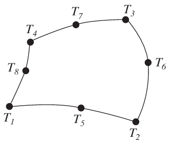
D.The evaluation of the integrals for the 2D isoparametric 8 node element is based on a temperature approximation \(T(\xi, \eta)\), expressed in a local coordinates system in terms of the nodal variables \(T_1\) to \(T_8\) as
\[T(\xi, \eta) = \mathbf{N}^e \mathbf{a}^e\]where
\[\mathbf{N}^e = [\, N_1^e \;\; N_2^e \;\; N_3^e \;\; \dots \;\; N_8^e \,] \qquad \mathbf{a}^e = [\, T_1 \;\; T_2 \;\; T_3 \;\; \dots \;\; T_8 \,]^T\]The element shape functions are given by
\[\begin{split}\begin{aligned} N_1^e &= -\frac{1}{4}(1-\xi)(1-\eta)(1+\xi+\eta) & N_5^e &= \frac{1}{2}(1-\xi^2)(1-\eta) \\ N_2^e &= -\frac{1}{4}(1+\xi)(1-\eta)(1-\xi+\eta) & N_6^e &= \frac{1}{2}(1+\xi)(1-\eta^2) \\ N_3^e &= -\frac{1}{4}(1+\xi)(1+\eta)(1-\xi-\eta) & N_7^e &= \frac{1}{2}(1-\xi^2)(1+\eta) \\ N_4^e &= -\frac{1}{4}(1-\xi)(1+\eta)(1+\xi-\eta) & N_8^e &= \frac{1}{2}(1-\xi)(1-\eta^2) \end{aligned}\end{split}\]The \(\mathbf{B}^e\)-matrix is given by
\[\begin{split}\mathbf{B}^e = \nabla \mathbf{N}^e = \begin{bmatrix} \frac{\partial}{\partial x} \\ \frac{\partial}{\partial y} \end{bmatrix} \mathbf{N}^e = (\mathbf{J}^T)^{-1} \begin{bmatrix} \frac{\partial}{\partial \xi} \\ \frac{\partial}{\partial \eta} \end{bmatrix} \mathbf{N}^e\end{split}\]where \(\mathbf{J}\) is the Jacobian matrix
\[\begin{split}\mathbf{J} = \begin{bmatrix} \frac{\partial x}{\partial \xi} & \frac{\partial x}{\partial \eta} \\ \frac{\partial y}{\partial \xi} & \frac{\partial y}{\partial \eta} \end{bmatrix}\end{split}\]Evaluation of the integrals is done by Gauss integration.
flw2i8s
- Purpose:
Compute heat flux and temperature gradients in an 8 node isoparametric heat flow element.
- Syntax:
[es, et, eci] = flw2i8s(ex, ey, ep, D, ed)- Description:
flw2i8scomputes the heat flux vectoresand the temperature gradientet(or corresponding quantities) in an 8 node isoparametric heat flow element.The input variables
ex,ey,epand the matrixDare defined inflw2i8e. The vectoredcontains the nodal temperatures \(\mathbf{a}^e\) of the element and is obtained by the functionextractas\[\mathbf{ed} = (\mathbf{a}^e)^T = [\;T_1\;\; T_2\;\; T_3\;\;\dots\;\, T_8\;]\]The output variables
\[\begin{split}\mathbf{es} = \bar{\mathbf{q}}^T = \left[ \begin{array}{cc} q^1_x & q^1_y \\ q^2_x & q^2_y \\ \vdots & \vdots \\ q^{n^2}_x & q^{n^2}_y \end{array} \right]\end{split}\]\[\begin{split}\mathbf{et} = (\bar {\nabla} T)^T = \left[ \begin{array}{cc} \frac{\partial T}{\partial x}^1 & \frac{\partial T}{\partial y}^1 \\ \frac{\partial T}{\partial x}^2 & \frac{\partial T}{\partial y}^2 \\ \vdots & \vdots \\ \frac{\partial T}{\partial x}^{n^2} & \frac{\partial T}{\partial y}^{n^2} \end{array} \right]\end{split}\]\[\begin{split}\mathbf{eci} = \left[ \begin{array}{cc} x_1 & y_1 \\ x_2 & y_2 \\ \vdots & \vdots \\ x_{n^2} & y_{n^2} \end{array} \right]\end{split}\]contain the heat flux, the temperature gradient, and the coordinates of the integration points. The index \(n\) denotes the number of integration points used within the element, see
flw2i8e.- Theory:
The temperature gradient and the heat flux are computed according to
\[\nabla T = \mathbf{B}^e\,\mathbf{a}^e\]\[\mathbf{q} = - \mathbf{D} \nabla T\]where the matrices \(\mathbf{D}\), \(\mathbf{B}^e\), and \(\mathbf{a}^e\) are described in
flw2i8e, and where the integration points are chosen as evaluation points.
flw3i8e
- Purpose:
Compute element stiffness matrix for an 8 node isoparametric element.

- Syntax:
Ke = flw3i8e(ex, ey, ez, ep, D) [Ke, fe] = flw3i8e(ex, ey, ez, ep, D, eq)- Description:
flw3i8eprovides the element stiffness (conductivity) matrixKeand the element load vectorfefor an 8 node isoparametric heat flow element.The element nodal coordinates \(x_1\), \(y_1\), \(z_1\), \(x_2\) etc, are supplied to the function by
ex,eyandez. The number of Gauss points \(n\) (\(n \times n \times n\) integration points, \(n=1,2,3\)) are supplied to the function byepand the thermal conductivities (or corresponding quantities) \(k_{xx}\), \(k_{xy}\) etc are supplied byD.\[\begin{split}\begin{array}{l} \mathbf{ex} = [\, x_1 \;\; x_2 \;\; x_3 \;\; \dots \;\; x_8 \,] \\ \mathbf{ey} = [\, y_1 \;\; y_2 \;\; y_3 \;\; \dots \;\; y_8 \,] \\ \mathbf{ez} = [\, z_1 \;\; z_2 \;\; z_3 \;\; \dots \;\; z_8 \,] \end{array} \qquad \mathbf{ep} = [\, n \,] \qquad \mathbf{D} = \begin{bmatrix} k_{xx} & k_{xy} & k_{xz} \\ k_{yx} & k_{yy} & k_{yz} \\ k_{zx} & k_{zy} & k_{zz} \end{bmatrix}\end{split}\]If the scalar variable
eqis given in the function, the element load vector \(\mathbf{fe}\) is computed, using\[\mathbf{eq} = [\, Q \,]\]where \(Q\) is the heat supply per unit volume.
- Theory:
The element stiffness matrix \(\mathbf{K}^e\) and the element load vector \(\mathbf{f}_l^e\), stored in
Keandfe, respectively, are computed according to\[ \begin{align}\begin{aligned}\mathbf{K}^e = \int_V \mathbf{B}^{eT} \mathbf{D} \mathbf{B}^e \, dV\\\mathbf{f}_l^e = \int_V \mathbf{N}^{eT} Q \, dV\end{aligned}\end{align} \]with the constitutive matrix \(\mathbf{D}\) defined by
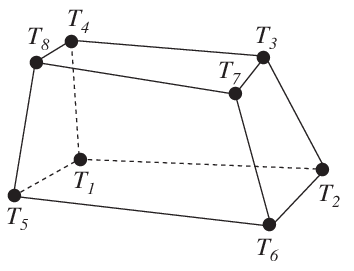
D.The evaluation of the integrals for the 3D isoparametric 8 node element is based on a temperature approximation \(T(\xi, \eta, \zeta)\), expressed in a local coordinate system in terms of the nodal variables \(T_1\) to \(T_8\) as
\[ \begin{align}\begin{aligned}T(\xi, \eta, \zeta) = \mathbf{N}^e \mathbf{a}^e\\\mathbf{N}^e = [\, N_1^e \;\; N_2^e \;\; N_3^e \;\; \dots \;\; N_8^e \,] \qquad \mathbf{a}^e = [\, T_1 \;\; T_2 \;\; T_3 \;\; \dots \;\; T_8 \,]^T\end{aligned}\end{align} \]The element shape functions are given by
\[\begin{split}N_1^e = \frac{1}{8}(1-\xi)(1-\eta)(1-\zeta) \qquad N_2^e = \frac{1}{8}(1+\xi)(1-\eta)(1-\zeta) \\ N_3^e = \frac{1}{8}(1+\xi)(1+\eta)(1-\zeta) \qquad N_4^e = \frac{1}{8}(1-\xi)(1+\eta)(1-\zeta) \\ N_5^e = \frac{1}{8}(1-\xi)(1-\eta)(1+\zeta) \qquad N_6^e = \frac{1}{8}(1+\xi)(1-\eta)(1+\zeta) \\ N_7^e = \frac{1}{8}(1+\xi)(1+\eta)(1+\zeta) \qquad N_8^e = \frac{1}{8}(1-\xi)(1+\eta)(1+\zeta)\end{split}\]The \(\mathbf{B}^e\)-matrix is given by
\[\begin{split}\mathbf{B}^e = \nabla \mathbf{N}^e = \begin{bmatrix} \frac{\partial}{\partial x} \\ \frac{\partial}{\partial y} \\ \frac{\partial}{\partial z} \end{bmatrix} \mathbf{N}^e = (\mathbf{J}^T)^{-1} \begin{bmatrix} \frac{\partial}{\partial \xi} \\ \frac{\partial}{\partial \eta} \\ \frac{\partial}{\partial \zeta} \end{bmatrix} \mathbf{N}^e\end{split}\]where \(\mathbf{J}\) is the Jacobian matrix
\[\begin{split}\mathbf{J} = \begin{bmatrix} \frac{\partial x}{\partial \xi} & \frac{\partial x}{\partial \eta} & \frac{\partial x}{\partial \zeta} \\ \frac{\partial y}{\partial \xi} & \frac{\partial y}{\partial \eta} & \frac{\partial y}{\partial \zeta} \\ \frac{\partial z}{\partial \xi} & \frac{\partial z}{\partial \eta} & \frac{\partial z}{\partial \zeta} \end{bmatrix}\end{split}\]Evaluation of the integrals is done by Gauss integration.
flw3i8s
- Purpose:
Compute heat flux and temperature gradients in an 8 node isoparametric heat flow element.
- Syntax:
[es, et, eci] = flw3i8s(ex, ey, ez, ep, D, ed)- Description:
flw3i8scomputes the heat flux vectoresand the temperature gradientet(or corresponding quantities) in an 8 node isoparametric heat flow element.The input variables \(\mathbf{ex}\), \(\mathbf{ey}\), \(\mathbf{ez}\), \(\mathbf{ep}\) and the matrix \(\mathbf{D}\) are defined in
flw3i8e. The vector \(\mathbf{ed}\) contains the nodal temperatures \(\mathbf{a}^e\) of the element and is obtained by the functionextractas\[\mathbf{ed} = (\mathbf{a}^e)^T = [\,T_1\;\; T_2\;\; T_3\;\;\dots\;\; T_8\,]\]The output variables
\[\begin{split}\mathbf{es} = \bar{\mathbf{q}}^T = \begin{bmatrix} q^1_x & q^1_y & q^1_z \\ q^2_x & q^2_y & q^2_z \\ \vdots & \vdots & \vdots\\ q^{n^3}_x & q^{n^3}_y & q^{n^3}_z \end{bmatrix}\end{split}\]\[\begin{split}\mathbf{et} = (\bar {\nabla} T)^T = \begin{bmatrix} \frac{\partial T}{\partial x}^1 & \frac{\partial T}{\partial y}^1 & \frac{\partial T}{\partial z}^1\\ \frac{\partial T}{\partial x}^2 & \frac{\partial T}{\partial y}^2 & \frac{\partial T}{\partial z}^2\\ \vdots & \vdots & \vdots \\ \frac{\partial T}{\partial x}^{n^3} & \frac{\partial T}{\partial y}^{n^3} & \frac{\partial T}{\partial z}^{n^3} \end{bmatrix} \qquad \mathbf{eci} = \begin{bmatrix} x_1 & y_1 & z_1 \\ x_2 & y_2 & z_2 \\ \vdots & \vdots & \vdots \\ x_{n^3} & y_{n^3} & z_{n^3} \end{bmatrix}\end{split}\]contain the heat flux, the temperature gradient, and the coordinates of the integration points. The index \(n\) denotes the number of integration points used within the element, see
flw3i8e.- Theory:
The temperature gradient and the heat flux are computed according to
\[\nabla T = \mathbf{B}^e\,\mathbf{a}^e\]\[\mathbf{q} = - \mathbf{D} \nabla T\]where the matrices \(\mathbf{D}\), \(\mathbf{B}^e\), and \(\mathbf{a}^e\) are described in
flw3i8e, and where the integration points are chosen as evaluation points.
Solid elements functions
Solid elements are available for two dimensional analysis in plane stress (panels) and plane strain, and for general three dimensional analysis. In the two dimensional case there are a triangular three node element, a quadrilateral four node element, two rectangular four node elements, and quadrilateral isoparametric four and eight node elements. For three dimensional analysis there is an eight node isoparametric element.
The elements are able to deal with both isotropic and anisotropic materials. The triangular element and the three isoparametric elements can also be used together with a nonlinear material model.
The material properties are specified by supplying the constitutive matrix \(\mathbf{D}\) as an input variable to the element functions. This matrix can be formed by the functions described in Section Material functions.
|
|
|
|
|
|
plante |
Compute element matrices for a triangular element |
plants |
Compute stresses and strains |
plantf |
Compute internal element forces |
planqe |
Compute element matrices for a quadrilateral element |
planqs |
Compute stresses and strains |
planre |
Compute element matrices for a rectangular Melosh element |
planrs |
Compute stresses and strains |
plantce |
Compute element matrices for a rectangular Turner-Clough element |
plantcs |
Compute stresses and strains |
plani4e |
Compute element matrices, 4 node isoparametric element |
plani4s |
Compute stresses and strains |
plani4f |
Compute internal element forces |
plani8e |
Compute element matrices, 8 node isoparametric element |
plani8s |
Compute stresses and strains |
plani8f |
Compute internal element forces |
soli8e |
Compute element matrices, 8 node isoparametric element |
soli8s |
Compute stresses and strains |
soli8f |
Compute internal element forces |
plante
- Purpose:
Compute element matrices for a triangular element in plane strain or plane stress.

- Syntax:
Ke = plante(ex, ey, ep, D) [Ke, fe] = plante(ex, ey, ep, D, eq)- Description:
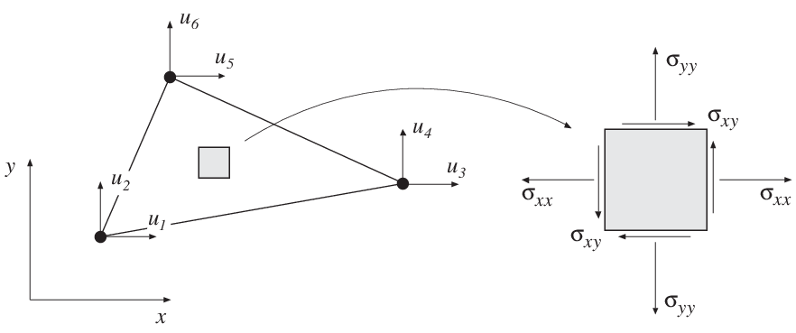
planteprovides an element stiffness matrixKeand an element load vectorfefor a triangular element in plane strain or plane stress.The element nodal coordinates \(x_1, y_1, x_2, \ldots\) are supplied to the function by \(\mathbf{ex}\) and \(\mathbf{ey}\). The type of analysis
ptypeand the element thicknesstare supplied by \(\mathbf{ep}\),\[\begin{split}\begin{array}{l} ptype=1 \quad \text{plane stress} \\ ptype=2 \quad \text{plane strain} \end{array}\end{split}\]and the material properties are supplied by the constitutive matrix
D. Any arbitrary \(\mathbf{D}\)-matrix with dimensions from \(3 \times 3\) to \(6 \times 6\) may be given. For an isotropic elastic material the constitutive matrix can be formed by the functionhooke, see Section Material functions.\[\begin{split}\mathbf{ex} = [\,x_1 \;\; x_2 \;\; x_3\,] \\ \mathbf{ey} = [\,y_1 \;\; y_2 \;\; y_3\,] \\ \mathbf{ep} = [\,ptype \;\; t\,]\end{split}\]\[\begin{split}\mathbf{D} = \begin{bmatrix} D_{11} & D_{12} & D_{13} \\ D_{21} & D_{22} & D_{23} \\ D_{31} & D_{32} & D_{33} \end{bmatrix} \quad \text{or} \quad \mathbf{D} = \begin{bmatrix} D_{11} & D_{12} & D_{13} & D_{14} & [D_{15}] & [D_{16}] \\ D_{21} & D_{22} & D_{23} & D_{24} & [D_{25}] & [D_{26}] \\ D_{31} & D_{32} & D_{33} & D_{34} & [D_{35}] & [D_{36}] \\ D_{41} & D_{42} & D_{43} & D_{44} & [D_{45}] & [D_{46}] \\ [D_{51}] & [D_{52}] & [D_{53}] & [D_{54}] & [D_{55}] & [D_{56}] \\ [D_{61}] & [D_{62}] & [D_{63}] & [D_{64}] & [D_{65}] & [D_{66}] \end{bmatrix}\end{split}\]If uniformly distributed loads are applied to the element, the element load vector
feis computed. The input variable\[\begin{split}\text{eq} = \begin{bmatrix} b_x \\ b_y \end{bmatrix}\end{split}\]containing loads per unit volume, \(b_x\) and \(b_y\), is then given.
- Theory:
The element stiffness matrix \(\mathbf{K}^e\) and the element load vector \(\mathbf{f}_l^e\), stored in
Keandfe, respectively, are computed according to\[\mathbf{K}^e = (\mathbf{C}^{-1})^T \int_A \bar{\mathbf{B}}^T \mathbf{D} \bar{\mathbf{B}}\, t\, dA\, \mathbf{C}^{-1}\]\[\mathbf{f}_l^e = (\mathbf{C}^{-1})^T \int_A \bar{\mathbf{N}}^T \mathbf{b}\, t\, dA\]with the constitutive matrix \(\mathbf{D}\) defined by
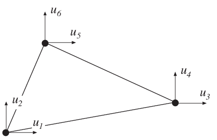
D, and the body force vector \(\mathbf{b}\) defined byeq.The evaluation of the integrals for the triangular element is based on a linear displacement approximation \(\mathbf{u}(x, y)\) and is expressed in terms of the nodal variables \(u_1, u_2, \ldots, u_6\) as
\[\mathbf{u}(x, y) = \mathbf{N}^e \mathbf{a}^e = \bar{\mathbf{N}}\, \mathbf{C}^{-1} \mathbf{a}^e\]where
\[\begin{split}\mathbf{u} = \begin{bmatrix} u_x \\ u_y \end{bmatrix} \quad \bar{\mathbf{N}} = \begin{bmatrix} 1 & x & y & 0 & 0 & 0 \\ 0 & 0 & 0 & 1 & x & y \end{bmatrix}\end{split}\]\[\begin{split}\mathbf{C} = \begin{bmatrix} 1 & x_1 & y_1 & 0 & 0 & 0 \\ 0 & 0 & 0 & 1 & x_1 & y_1 \\ 1 & x_2 & y_2 & 0 & 0 & 0 \\ 0 & 0 & 0 & 1 & x_2 & y_2 \\ 1 & x_3 & y_3 & 0 & 0 & 0 \\ 0 & 0 & 0 & 1 & x_3 & y_3 \\ \end{bmatrix} \quad \mathbf{a}^e = \begin{bmatrix} u_1 \\ u_2 \\ u_3 \\ u_4 \\ u_5 \\ u_6 \end{bmatrix}\end{split}\]The matrix \(\bar{\mathbf{B}}\) is obtained as
\[\begin{split}\bar{\mathbf{B}} = \tilde{\nabla} \bar{\mathbf{N}} \quad \text{where} \quad \tilde{\nabla} = \begin{bmatrix} \dfrac{\partial}{\partial x} & 0 \\ 0 & \dfrac{\partial}{\partial y} \\ \dfrac{\partial}{\partial y} & \dfrac{\partial}{\partial x} \end{bmatrix}\end{split}\]If a larger \(\mathbf{D}\)-matrix than \(3 \times 3\) is used for plane stress (\(ptype=1\)), the \(\mathbf{D}\)-matrix is reduced to a \(3 \times 3\) matrix by static condensation using \(\sigma_{zz} = \sigma_{xz} = \sigma_{yz} = 0\). These stress components are connected with the rows 3, 5 and 6 in the D-matrix respectively.
If a larger \(\mathbf{D}\)-matrix than \(3 \times 3\) is used for plane strain (\(ptype=2\)), the \(\mathbf{D}\)-matrix is reduced to a \(3 \times 3\) matrix using \(\varepsilon_{zz} = \gamma_{xz} = \gamma_{yz} = 0\). This implies that a \(3 \times 3\) \(\mathbf{D}\)-matrix is created by the rows and the columns 1, 2 and 4 from the original D-matrix.
Evaluation of the integrals for the triangular element yields
\[\mathbf{K}^e = (\mathbf{C}^{-1})^T \bar{\mathbf{B}}^T \mathbf{D} \bar{\mathbf{B}}\, \mathbf{C}^{-1}\, t\, A\]\[\mathbf{f}_l^e = \frac{A t}{3} \begin{bmatrix} b_x & b_y & b_x & b_y & b_x & b_y \end{bmatrix}^T\]where the element area \(A\) is determined as
\[\begin{split}A = \frac{1}{2} \det \begin{bmatrix} 1 & x_1 & y_1 \\ 1 & x_2 & y_2 \\ 1 & x_3 & y_3 \end{bmatrix}\end{split}\]
plants
- Purpose:
Compute stresses and strains in a triangular element in plane strain or plane stress.
- Syntax:
[es, et] = plants(ex, ey, ep, D, ed)- Description:
plantscomputes the stressesesand the strainsetin a triangular element in plane strain or plane stress.The input variables \(\mathbf{ex}\), \(\mathbf{ey}\), \(\mathbf{ep}\) and \(\mathbf{D}\) are defined in
plante. The vector \(\mathbf{ed}\) contains the nodal displacements \(\mathbf{a}^e\) of the element and is obtained by the functionextractas\[\mathbf{ed} = (\mathbf{a}^e)^T = [\, u_1\;\; u_2\;\; \dots \;\; u_6\,]\]The output variables
\[\mathrm{es} = \boldsymbol{\sigma}^T = \left[\, \sigma_{xx}\; \sigma_{yy}\; [\sigma_{zz}]\; \sigma_{xy}\; [\sigma_{xz}]\; [\sigma_{yz}]\, \right]\]\[\mathrm{et} = \boldsymbol{\varepsilon}^T = [\, \varepsilon_{xx}\; \varepsilon_{yy}\; [\varepsilon_{zz}]\; \gamma_{xy}\; [\gamma_{xz}]\; [\gamma_{yz}]\,]\]contain the stress and strain components. The size of
esandetfollows the size ofD. Note that for plane stress \(\varepsilon_{zz} \neq 0\), and for plane strain \(\sigma_{zz} \neq 0\).- Theory:
The strains and stresses are computed according to
\[\boldsymbol{\varepsilon} = \bar{\mathbf{B}}\, \mathbf{C}^{-1}\, \mathbf{a}^e\]\[\boldsymbol{\sigma} = \mathbf{D}\, \boldsymbol{\varepsilon}\]where the matrices \(\mathbf{D}\), \(\bar{\mathbf{B}}\), \(\mathbf{C}\) and \(\mathbf{a}^e\) are described in
plante. Note that both the strains and the stresses are constant in the element.
plantf
- Purpose:
Compute internal element force vector in a triangular element in plane strain or plane stress.
- Syntax:
ef = plantf(ex, ey, ep, es)- Description:
plantfcomputes the internal element forcesefin a triangular element in plane strain or plane stress.The input variables \(\mathbf{ex}\), \(\mathbf{ey}\) and \(\mathbf{ep}\) are defined in
plante, and the input variable \(\mathbf{es}\) is defined inplants.The output variable
\[\mathrm{ef} = \mathbf{f}_i^{eT} = \left[\, f_{i1}\; f_{i2}\; \dots \; f_{i6}\; \right]\]contains the components of the internal force vector.
- Theory:
The internal force vector is computed according to
\[\mathbf{f}_i^e = (\mathbf{C}^{-1})^T \int_A \bar{\mathbf{B}}^T \boldsymbol{\sigma}\; t\; dA\]where the matrices \(\bar{\mathbf{B}}\) and \(\mathbf{C}\) are defined in
planteand \(\boldsymbol{\sigma}\) is defined inplants.Evaluation of the integral for the triangular element yields
\[\mathbf{f}_i^e = (\mathbf{C}^{-1})^T \bar{\mathbf{B}}^T\,\boldsymbol{\sigma}\; t\; A\]
planqe
- Purpose:
Compute element matrices for a quadrilateral element in plane strain or plane stress.

- Syntax:
Ke = planqe(ex, ey, ep, D) [Ke, fe] = planqe(ex, ey, ep, D, eq)- Description:
planqeprovides an element stiffness matrix \(Ke\) and an element load vector \(fe\) for a quadrilateral element in plane strain or plane stress.The element nodal coordinates \(x_1\), \(y_1\), \(x_2\), etc. are supplied to the function by \(\mathbf{ex}\) and \(\mathbf{ey}\). The type of analysis \(ptype\) and the element thickness \(t\) are supplied by \(\mathbf{ep}\):
\[\begin{split}\begin{array}{lll} ptype=1 & \quad \text{plane stress} \\ ptype=2 & \quad \text{plane strain} \end{array}\end{split}\]The material properties are supplied by the constitutive matrix \(D\). Any arbitrary \(\mathbf{D}\)-matrix with dimensions from \(3 \times 3\) to \(6 \times 6\) may be given. For an isotropic elastic material the constitutive matrix can be formed by the function
hooke, see Section Material functions.\[\begin{split}\mathbf{ex} = [\,x_1 \;\, x_2 \;\; x_3\;\, x_4\,] \\ \mathbf{ey} = [\,y_1 \;\,\, y_2 \;\; y_3\;\,\, y_4\,] \\ \mathbf{ep} = [\,ptype \;\, t\,]\end{split}\]\[\begin{split}\mathbf{D} = \begin{bmatrix} D_{11} & D_{12} & D_{13} \\ D_{21} & D_{22} & D_{23} \\ D_{31} & D_{32} & D_{33} \end{bmatrix} \quad \text{or} \quad \mathbf{D} = \begin{bmatrix} D_{11} & D_{12} & D_{13} & D_{14} & D_{15} & D_{16} \\ D_{21} & D_{22} & D_{23} & D_{24} & D_{25} & D_{26} \\ D_{31} & D_{32} & D_{33} & D_{34} & D_{35} & D_{36} \\ D_{41} & D_{42} & D_{43} & D_{44} & D_{45} & D_{46} \\ D_{51} & D_{52} & D_{53} & D_{54} & D_{55} & D_{56} \\ D_{61} & D_{62} & D_{63} & D_{64} & D_{65} & D_{66} \end{bmatrix}\end{split}\]If uniformly distributed loads are applied on the element, the element load vector \(fe\) is computed. The input variable
\[\begin{split}eq = \begin{bmatrix} b_x \\ b_y \end{bmatrix}\end{split}\]contains loads per unit volume, \(b_x\) and \(b_y\).
- Theory:
In computing the element matrices, two more degrees of freedom are introduced. The location of these two degrees of freedom is defined by the mean value of the coordinates at the corner points. Four sets of element matrices are calculated using
plante. These matrices are then assembled and the two extra degrees of freedom are eliminated by static condensation.
planqs
- Purpose:
Compute stresses and strains in a quadrilateral element in plane strain or plane stress.

- Syntax:
[es,et]=planqs(ex,ey,ep,D,ed) [es,et]=planqs(ex,ey,ep,D,ed,eq)- Description:
planqscomputes the stressesesand the strainsetin a quadrilateral element in plane strain or plane stress.The input variables \(\mathbf{ex}\), \(\mathbf{ey}\), \(\mathbf{ep}\), \(\mathbf{D}\) and \(\mathbf{eq}\) are defined in
planqe. The vector \(\mathbf{ed}\) contains the nodal displacements \(\mathbf{a}^e\) of the element and is obtained by the functionextractas\[\mathbf{ed} = (\mathbf{a}^e)^T = [\,u_1\;\; u_2\;\; \dots \;\; u_8\,]\]If body forces are applied to the element the variable \(\mathbf{eq}\) must be included.
The output variables
\[\mathrm{es} = \boldsymbol{\sigma}^T = [\, \sigma_{xx}\; \sigma_{yy}\; [\sigma_{zz}]\; \sigma_{xy}\; [\sigma_{xz}]\; [\sigma_{yz}]\,]\]\[\mathrm{et} = \boldsymbol{\varepsilon}^T = [\,\varepsilon_{xx}\;\varepsilon_{yy}\;[\varepsilon_{zz}]\;\gamma_{xy}\;[\gamma_{xz}]\;[\gamma_{yz}]\,]\]contain the stress and strain components. The size of
esandetfollows the size ofD. Note that for plane stress \(\varepsilon_{zz} \neq 0\), and for plane strain \(\sigma_{zz} \neq 0\).- Theory:
By assembling triangular elements as described in
planqea system of equations containing 10 degrees of freedom is obtained. From this system of equations the two unknown displacements at the center of the element are computed. Then according to the description inplantsthe strain and stress components in each of the four triangular elements are produced. Finally the quadrilateral element strains and stresses are computed as area weighted mean values from the values of the four triangular elements. If uniformly distributed loads are applied on the element, the element load vectoreqis needed for the calculations.
planre
- Purpose:
Compute element matrices for a rectangular (Melosh) element in plane strain or plane stress.

- Syntax:
Ke = planre(ex, ey, ep, D) [Ke, fe] = planre(ex, ey, ep, D, eq)- Description:
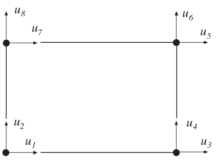
planre provides an element stiffness matrix Ke and an element load vector fe for a rectangular (Melosh) element in plane strain or plane stress. This element can only be used if the element edges are parallel to the coordinate axis.
The element nodal coordinates \((x_1, y_1)\) and \((x_3, y_3)\) are supplied to the function by ex and ey. The type of analysis ptype and the element thickness t are supplied by ep,
\[\begin{split}\begin{array}{lll} ptype=1 \quad \mbox{plane stress} \\ ptype=2 \quad \mbox{plane strain} \end{array}\end{split}\]and the material properties are supplied by the constitutive matrix D. Any arbitrary D-matrix with dimensions from \(3 \times 3\) to \(6 \times 6\) may be given. For an isotropic elastic material the constitutive matrix can be formed by the function hooke, see Section Material.
\[\begin{split}\begin{array}{l} \mathbf{ex} = [\,x_1 \;\, x_3\,] \\ \mathbf{ey} = [\,y_1 \;\, y_3\,] \end{array} \qquad \mathbf{ep} = [\,ptype \;\, t\,]\end{split}\]\[\begin{split}\mathbf{D} = \begin{bmatrix} D_{11} & D_{12} & D_{13} \\ D_{21} & D_{22} & D_{23} \\ D_{31} & D_{32} & D_{33} \end{bmatrix} \quad \text{or} \quad \mathbf{D} = \begin{bmatrix} D_{11} & D_{12} & D_{13} & D_{14} & [D_{15}] & [D_{16}] \\ D_{21} & D_{22} & D_{23} & D_{24} & [D_{25}] & [D_{26}] \\ D_{31} & D_{32} & D_{33} & D_{34} & [D_{35}] & [D_{36}] \\ D_{41} & D_{42} & D_{43} & D_{44} & [D_{45}] & [D_{46}] \\ [D_{51}] & [D_{52}] & [D_{53}] & [D_{54}] & [D_{55}] & [D_{56}] \\ [D_{61}] & [D_{62}] & [D_{63}] & [D_{64}] & [D_{65}] & [D_{66}] \end{bmatrix}\end{split}\]If uniformly distributed loads are applied on the element, the element load vector fe is computed. The input variable
\[\begin{split}eq = \begin{bmatrix} b_x \\ b_y \end{bmatrix}\end{split}\]containing loads per unit volume, \(b_x\) and \(b_y\), is then given.
- Theory:
The element stiffness matrix \(\mathbf{K}^e\) and the element load vector \(\mathbf{f}_l^e\), stored in Ke and fe, respectively, are computed according to
\[\mathbf{K}^e = \int_A \mathbf{B}^{eT} \mathbf{D} \mathbf{B}^e t\, dA\]\[\mathbf{f}_l^e = \int_A \mathbf{N}^{eT} \mathbf{b} t\, dA\]with the constitutive matrix \(\mathbf{D}\) defined by D, and the body force vector \(\mathbf{b}\) defined by eq.
The evaluation of the integrals for the rectangular element is based on a bilinear displacement approximation \(\mathbf{u}(x,y)\) and is expressed in terms of the nodal variables \(u_1, u_2, \dots, u_8\) as
\[\mathbf{u}(x, y) = \mathbf{N}^e \mathbf{a}^e\]where
\[\begin{split}\mathbf{u} = \begin{bmatrix} u_x \\ u_y \end{bmatrix} \quad \mathbf{N}^e = \begin{bmatrix} N^e_1 & 0 & N^e_2 & 0 & N^e_3 & 0 & N^e_4 & 0 \\ 0 & N^e_1 & 0 & N^e_2 & 0 & N^e_3 & 0 & N^e_4 \end{bmatrix} \quad \mathbf{a}^e = \begin{bmatrix} u_1 \\ u_2 \\ \vdots \\ u_8 \end{bmatrix}\end{split}\]With a local coordinate system located at the center of the element, the element shape functions \(N^e_1\)–\(N^e_4\) are obtained as
\[\begin{split}N^e_1 = \frac{1}{4ab}(x - x_2)(y - y_4) \\ N^e_2 = -\frac{1}{4ab}(x - x_1)(y - y_3) \\ N^e_3 = \frac{1}{4ab}(x - x_4)(y - y_2) \\ N^e_4 = -\frac{1}{4ab}(x - x_3)(y - y_1)\end{split}\]where
\[a = \frac{1}{2}(x_3 - x_1) \quad \text{and} \quad b = \frac{1}{2}(y_3 - y_1)\]The matrix \(\mathbf{B}^e\) is obtained as
\[\begin{split}\mathbf{B}^e = \tilde{\nabla} \mathbf{N}^e \qquad \text{where} \quad \tilde{\nabla} = \begin{bmatrix} \dfrac{\partial}{\partial x} & 0 \\ 0 & \dfrac{\partial}{\partial y} \\ \dfrac{\partial}{\partial y} & \dfrac{\partial}{\partial x} \end{bmatrix}\end{split}\]If a larger D-matrix than \(3 \\times 3\) is used for plane stress (\(ptype=1\)), the D-matrix is reduced to a \(3 \\times 3\) matrix by static condensation using \(\sigma_{zz} = \sigma_{xz} = \sigma_{yz} = 0\). These stress components are connected with the rows 3, 5 and 6 in the D-matrix respectively.
If a larger D-matrix than \(3 \\times 3\) is used for plane strain (\(ptype=2\)), the D-matrix is reduced to a \(3 \\times 3\) matrix using \(\varepsilon_{zz} = \gamma_{xz} = \gamma_{yz} = 0\). This implies that a \(3 \\times 3\) D-matrix is created by the rows and the columns 1, 2 and 4 from the original D-matrix.
Evaluation of the integrals for the rectangular element can be done either analytically or numerically by use of a \(2 \\times 2\) point Gauss integration. The element load vector \(\mathbf{f}_l^e\) yields
\[\begin{split}\mathbf{f}_l^e = abt \begin{bmatrix} b_x \\ b_y \\ b_x \\ b_y \\ b_x \\ b_y \\ b_x \\ b_y \end{bmatrix}\end{split}\]
planrs
- Purpose:
Compute stresses and strains in a rectangular (Melosh) element in plane strain or plane stress.

- Syntax:
[es,et]=planrs(ex,ey,ep,D,ed)- Description:
planrscomputes the stressesesand the strainsetin a rectangular (Melosh) element in plane strain or plane stress. The stress and strain components are computed at the center of the element.The input variables \(\mathbf{ex}\), \(\mathbf{ey}\), \(\mathbf{ep}\) and \(\mathbf{D}\) are defined in
planre. The vector \(\mathbf{ed}\) contains the nodal displacements \(\mathbf{a}^e\) of the element and is obtained by the functionextractas\[\mathbf{ed} = (\mathbf{a}^e)^T = [\,u_1\;\; u_2\;\; \dots \;\; u_8\,]\]The output variables
\[\mathrm{es} = \boldsymbol{\sigma}^T = [\, \sigma_{xx}\; \sigma_{yy}\; [\sigma_{zz}]\; \sigma_{xy}\; [\sigma_{xz}]\; [\sigma_{yz}]\,]\]\[\mathrm{et} = \boldsymbol{\varepsilon}^T = [\, \varepsilon_{xx}\; \varepsilon_{yy}\; [\varepsilon_{zz}]\; \gamma_{xy}\; [\gamma_{xz}]\; [\gamma_{yz}]\,]\]contain the stress and strain components. The size of
esandetfollows the size ofD. Note that for plane stress \(\varepsilon_{zz} \neq 0\), and for plane strain \(\sigma_{zz} \neq 0\).- Theory:
The strains and stresses are computed according to
\[\boldsymbol{\varepsilon} = \mathbf{B}^e\,\mathbf{a}^e\]\[\boldsymbol{\sigma} = \mathbf{D}\,\boldsymbol{\varepsilon}\]where the matrices \(\mathbf{D}\), \(\mathbf{B}^e\), and \(\mathbf{a}^e\) are described in
planre, and where the evaluation point \((x, y)\) is chosen to be at the center of the element.
plantce
- Purpose:
Compute element matrices for a rectangular (Turner-Clough) element in plane strain or plane stress.
- Syntax:
Ke = plantce(ex, ey, ep) [Ke, fe] = plantce(ex, ey, ep, eq)- Description:
plantceprovides an element stiffness matrixKeand an element load vectorfefor a rectangular (Turner-Clough) element in plane strain or plane stress. This element can only be used if the material is isotropic and if the element edges are parallel to the coordinate axis.The element nodal coordinates \((x_1, y_1)\) and \((x_3, y_3)\) are supplied to the function by \(\mathbf{ex}\) and \(\mathbf{ey}\). The state of stress
ptype, the element thickness \(t\) and the material properties \(E\) and \(\nu\) are supplied by \(\mathbf{ep}\). For plane stress \(ptype=1\) and for plane strain \(ptype=2\).\[\begin{split}\begin{array}{l} \mathbf{ex} = [\, x_1 \;\; x_3\,] \\ \mathbf{ey} = [\, y_1 \;\; y_3\,] \end{array} \qquad \mathbf{ep} = [\, ptype \;\; t \;\; E \;\; \nu \,]\end{split}\]If uniformly distributed loads are applied to the element, the element load vector
feis computed. The input variable\[\begin{split}eq = \begin{bmatrix} b_x \\ b_y \end{bmatrix}\end{split}\]containing loads per unit volume, \(b_x\) and \(b_y\), is then given.
- Theory:
The element stiffness matrix \(\mathbf{K}^e\) and the element load vector \(\mathbf{f}_l^e\), stored in
Keandfe, respectively, are computed according to\[\mathbf{K}^e = \int_A \mathbf{B}^{eT} \mathbf{D} \mathbf{B}^e t\, dA\]\[\mathbf{f}_l^e = \int_A \mathbf{N}^{eT} \mathbf{b} t\, dA\]where the constitutive matrix \(\mathbf{D}\) is described in
hooke, see Section Material functions, and the body force vector \(\mathbf{b}\) is defined byeq.The evaluation of the integrals for the Turner-Clough element is based on a displacement field \(\mathbf{u}(x, y)\) built up of a bilinear displacement approximation superposed by bubble functions in order to create a linear stress field over the element. The displacement field is expressed in terms of the nodal variables \(u_1, u_2, \dots, u_8\) as
\[\mathbf{u}(x, y) = \mathbf{N}^e \mathbf{a}^e\]where
\[\begin{split}\mathbf{u} = \begin{bmatrix} u_x \\ u_y \end{bmatrix} \quad \mathbf{N}^e = \begin{bmatrix} N^e_1 & N^e_5 & N^e_2 & -N^e_5 & N^e_3 & N^e_5 & N^e_4 & -N^e_5 \\ N^e_6 & N^e_1 & -N^e_6 & N^e_2 & N^e_6 & N^e_3 & -N^e_6 & N^e_4 \end{bmatrix} \quad \mathbf{a}^e = \begin{bmatrix} u_1 \\ u_2 \\ \vdots \\ u_8 \end{bmatrix}\end{split}\]With a local coordinate system located at the center of the element, the element shape functions \(N^e_1\)–\(N^e_6\) are obtained as
\[\begin{split}N^e_1 = \frac{1}{4ab}(a-x)(b-y) \\ N^e_2 = \frac{1}{4ab}(a+x)(b-y) \\ N^e_3 = \frac{1}{4ab}(a+x)(b+y) \\ N^e_4 = \frac{1}{4ab}(a-x)(b+y) \\ N^e_5 = \frac{1}{8ab}\left[ (b^2-y^2) + \nu (a^2-x^2) \right] \\ N^e_6 = \frac{1}{8ab}\left[ (a^2-x^2) + \nu (b^2-y^2) \right]\end{split}\]where
\[a = \frac{1}{2}(x_3 - x_1) \qquad b = \frac{1}{2}(y_3 - y_1)\]The matrix \(\mathbf{B}^e\) is obtained as
\[\begin{split}\mathbf{B}^e = \tilde{\nabla} \mathbf{N}^e \qquad \text{where} \quad \tilde{\nabla} = \begin{bmatrix} \dfrac{\partial}{\partial x} & 0 \\ 0 & \dfrac{\partial}{\partial y} \\ \dfrac{\partial}{\partial y} & \dfrac{\partial}{\partial x} \end{bmatrix}\end{split}\]Evaluation of the integrals for the Turner-Clough element can be done either analytically or numerically by use of a \(2 \times 2\) point Gauss integration. The element load vector \(\mathbf{f}_l^e\) yields
\[\begin{split}\mathbf{f}_l^e = abt \begin{bmatrix} b_x \\ b_y \\ b_x \\ b_y \\ b_x \\ b_y \\ b_x \\ b_y \end{bmatrix}\end{split}\]
plantcs
- Purpose:
Compute stresses and strains in a Turner-Clough element in plane strain or plane stress.
- Syntax:
[es, et] = plantcs(ex, ey, ep, ed)- Description:
plantcscomputes the stressesesand the strainsetin a rectangular Turner-Clough element in plane strain or plane stress. The stress and strain components are computed at the center of the element.The input variables \(\mathbf{ex}\), \(\mathbf{ey}\), and \(\mathbf{ep}\) are defined in
plantce. The vector \(\mathbf{ed}\) contains the nodal displacements \(\mathbf{a}^e\) of the element and is obtained by the functionextractas\[\mathbf{ed} = (\mathbf{a}^e)^T = [\, u_1\;\; u_2\;\; \dots \;\; u_8\,]\]The output variables
\[\mathrm{es} = \boldsymbol{\sigma}^T = [\, \sigma_{xx}\; \sigma_{yy}\; [\sigma_{zz}]\; \sigma_{xy}\; [\sigma_{xz}]\; [\sigma_{yz}]\,]\]\[\mathrm{et} = \boldsymbol{\varepsilon}^T = [\, \varepsilon_{xx}\; \varepsilon_{yy}\; [\varepsilon_{zz}]\; \gamma_{xy}\; [\gamma_{xz}]\; [\gamma_{yz}]\,]\]contain the stress and strain components. The size of
esandetfollows the size ofD. Note that for plane stress \(\varepsilon_{zz} \neq 0\), and for plane strain \(\sigma_{zz} \neq 0\).- Theory:
The strains and stresses are computed according to
\[\boldsymbol{\varepsilon} = \mathbf{B}^e\,\mathbf{a}^e\]\[\boldsymbol{\sigma} = \mathbf{D}\;\boldsymbol{\varepsilon}\]where the matrices \(\mathbf{D}\), \(\mathbf{B}^e\), and \(\mathbf{a}^e\) are described in
plantce, and where the evaluation point \((x, y)\) is chosen to be at the center of the element.
plani4e
- Purpose:
Compute element matrices for a 4 node isoparametric element in plane strain or plane stress.
- Syntax:
Ke = plani4e(ex, ey, ep, D) [Ke, fe] = plani4e(ex, ey, ep, D, eq)- Description:
plani4eprovides an element stiffness matrixKeand an element load vectorfefor a 4 node isoparametric element in plane strain or plane stress.The element nodal coordinates \(x_1, y_1, x_2, \ldots\) are supplied to the function by \(\mathbf{ex}\) and \(\mathbf{ey}\). The type of analysis \(ptype\), the element thickness \(t\), and the number of Gauss points \(n\) are supplied by \(\mathbf{ep}\):
\[\begin{split}\begin{array}{lll} ptype=1 & \text{plane stress} & (n \times n) \text{ integration points} \\ ptype=2 & \text{plane strain} & n=1,2,3 \end{array}\end{split}\]The material properties are supplied by the constitutive matrix \(D\). Any arbitrary \(\mathbf{D}\)-matrix with dimensions from \(3 \times 3\) to \(6 \times 6\) may be given. For an isotropic elastic material the constitutive matrix can be formed by the function
hooke, see Section Material functions.\[\begin{split}\mathbf{ex} = [\,x_1 \;\, x_2 \;\; x_3\;\, x_4\,] \\ \mathbf{ey} = [\,y_1 \;\,\, y_2 \;\; y_3\;\,\, y_4\,] \\ \mathbf{ep} = [\,ptype \;\, t\;\, n\,]\end{split}\]\[\begin{split}\mathbf{D} = \begin{bmatrix} D_{11} & D_{12} & D_{13} \\ D_{21} & D_{22} & D_{23} \\ D_{31} & D_{32} & D_{33} \end{bmatrix} \quad \text{or} \quad \mathbf{D} = \begin{bmatrix} D_{11} & D_{12} & D_{13} & D_{14} & [D_{15}] & [D_{16}] \\ D_{21} & D_{22} & D_{23} & D_{24} & [D_{25}] & [D_{26}] \\ D_{31} & D_{32} & D_{33} & D_{34} & [D_{35}] & [D_{36}] \\ D_{41} & D_{42} & D_{43} & D_{44} & [D_{45}] & [D_{46}] \\ [D_{51}] & [D_{52}] & [D_{53}] & [D_{54}] & [D_{55}] & [D_{56}] \\ [D_{61}] & [D_{62}] & [D_{63}] & [D_{64}] & [D_{65}] & [D_{66}] \end{bmatrix}\end{split}\]If different \(\mathbf{D}_i\) matrices are used in the Gauss points, these \(\mathbf{D}_i\) matrices are stored in a global vector
D. For numbering of the Gauss points, seeeciinplani4s.\[\begin{split}\mathbf{D} = \begin{bmatrix} \mathbf{D}_1 \\ \mathbf{D}_2 \\ \vdots \\ \mathbf{D}_{n^2} \end{bmatrix}\end{split}\]If uniformly distributed loads are applied to the element, the element load vector
feis computed. The input variable\[\begin{split}\mathrm{eq} = \begin{bmatrix} b_x \\ b_y \end{bmatrix}\end{split}\]containing loads per unit volume, \(b_x\) and \(b_y\), is then given.
- Theory:
The element stiffness matrix \(\mathbf{K}^e\) and the element load vector \(\mathbf{f}_l^e\), stored in
Keandfe, respectively, are computed according to\[\begin{split}\mathbf{K}^e = \int_A \mathbf{B}^{eT} \mathbf{D} \mathbf{B}^e t\, dA \\ \mathbf{f}_l^e = \int_A \mathbf{N}^{eT} \mathbf{b} t\, dA\end{split}\]with the constitutive matrix \(\mathbf{D}\) defined by
D, and the body force vector \(\mathbf{b}\) defined byeq.The evaluation of the integrals for the isoparametric 4 node element is based on a displacement approximation \(\mathbf{u}(\xi, \eta)\), expressed in a local coordinate system in terms of the nodal variables \(u_1, u_2, \ldots, u_8\) as
\[\mathbf{u}(\xi, \eta) = \mathbf{N}^e \mathbf{a}^e\]where
\[\begin{split}\mathbf{u} = \begin{bmatrix} u_x \\ u_y \end{bmatrix} \qquad \mathbf{N}^e = \begin{bmatrix} N_1^e & 0 & N_2^e & 0 & N_3^e & 0 & N_4^e & 0 \\ 0 & N_1^e & 0 & N_2^e & 0 & N_3^e & 0 & N_4^e \end{bmatrix} \qquad \mathbf{a}^e = \begin{bmatrix} u_1 \\ u_2 \\ \vdots \\ u_8 \end{bmatrix}\end{split}\]The element shape functions are given by
\[\begin{split}N_1^e = \frac{1}{4}(1-\xi)(1-\eta) \qquad N_2^e = \frac{1}{4}(1+\xi)(1-\eta) \\ N_3^e = \frac{1}{4}(1+\xi)(1+\eta) \qquad N_4^e = \frac{1}{4}(1-\xi)(1+\eta)\end{split}\]The matrix \(\mathbf{B}^e\) is obtained as
\[\begin{split}\mathbf{B}^e = \tilde{\nabla} \mathbf{N}^e \qquad \text{where} \quad \tilde{\nabla} = \begin{bmatrix} \frac{\partial}{\partial x} & 0 \\ 0 & \frac{\partial}{\partial y} \\ \frac{\partial}{\partial y} & \frac{\partial}{\partial x} \end{bmatrix}\end{split}\]and
\[\begin{split}\begin{bmatrix} \frac{\partial}{\partial x} \\ \frac{\partial}{\partial y} \end{bmatrix} = (\mathbf{J}^T)^{-1} \begin{bmatrix} \frac{\partial}{\partial \xi} \\ \frac{\partial}{\partial \eta} \end{bmatrix} \qquad \mathbf{J} = \begin{bmatrix} \frac{\partial x}{\partial \xi} & \frac{\partial x}{\partial \eta} \\ \frac{\partial y}{\partial \xi} & \frac{\partial y}{\partial \eta} \end{bmatrix}\end{split}\]If a larger \(\mathbf{D}\)-matrix than \(3 \times 3\) is used for plane stress (\(ptype=1\)), the \(\mathbf{D}\)-matrix is reduced to a \(3 \times 3\) matrix by static condensation using \(\sigma_{zz} = \sigma_{xz} = \sigma_{yz} = 0\). These stress components are connected with the rows 3, 5 and 6 in the D-matrix respectively.
If a larger \(\mathbf{D}\)-matrix than \(3 \times 3\) is used for plane strain (\(ptype=2\)), the \(\mathbf{D}\)-matrix is reduced to a \(3 \times 3\) matrix using \(\varepsilon_{zz} = \gamma_{xz} = \gamma_{yz} = 0\). This implies that a \(3 \times 3\) \(\mathbf{D}\)-matrix is created by the rows and the columns 1, 2 and 4 from the original D-matrix.
Evaluation of the integrals is done by Gauss integration.
plani4s
- Purpose:
Compute stresses and strains in a 4 node isoparametric element in plane strain or plane stress.
- Syntax:
[es,et,eci]=plani4s(ex,ey,ep,D,ed)- Description:
plani4scomputes stressesesand the strainsetin a 4 node isoparametric element in plane strain or plane stress.The input variables \(\mathbf{ex}\), \(\mathbf{ey}\), \(\mathbf{ep}\) and the matrix \(\mathbf{D}\) are defined in
plani4e. The vector \(\mathbf{ed}\) contains the nodal displacements \(\mathbf{a}^e\) of the element and is obtained by the functionextractas\[\mathbf{ed} = (\mathbf{a}^e)^T = [\,u_1\;\; u_2\;\; \dots \;\; u_8\,]\]The output variables
\[\begin{split}\mathrm{es} = \boldsymbol{\sigma}^T = \begin{bmatrix} \sigma^1_{xx} & \sigma^1_{yy} & [\sigma^1_{zz}] & \sigma^1_{xy} & [\sigma^1_{xz}] & [\sigma^1_{yz}] \\ \sigma^2_{xx} & \sigma^2_{yy} & [\sigma^2_{zz}] & \sigma^2_{xy} & [\sigma^2_{xz}] & [\sigma^2_{yz}] \\ \vdots & \vdots & \vdots & \vdots & \vdots & \vdots \\ \sigma^{n^2}_{xx} & \sigma^{n^2}_{yy} & [\sigma^{n^2}_{zz}] & \sigma^{n^2}_{xy} & [\sigma^{n^2}_{xz}] & [\sigma^{n^2}_{yz}] \end{bmatrix}\end{split}\]\[\begin{split}\mathrm{et} = \boldsymbol{\varepsilon}^T = \begin{bmatrix} \varepsilon^1_{xx} & \varepsilon^1_{yy} & [\varepsilon^1_{zz}] & \gamma^1_{xy} & [\gamma^1_{xz}] & [\gamma^1_{yz}] \\ \varepsilon^2_{xx} & \varepsilon^2_{yy} & [\varepsilon^2_{zz}] & \gamma^2_{xy} & [\gamma^2_{xz}] & [\gamma^2_{yz}] \\ \vdots & \vdots & \vdots & \vdots & \vdots & \vdots \\ \varepsilon^{n^2}_{xx} & \varepsilon^{n^2}_{yy} & [\varepsilon^{n^2}_{zz}] & \gamma^{n^2}_{xy} & [\gamma^{n^2}_{xz}] & [\gamma^{n^2}_{yz}] \end{bmatrix}\end{split}\]\[\begin{split}\mathbf{eci} = \begin{bmatrix} x_1 & y_1 \\ x_2 & y_2 \\ \vdots & \vdots \\ x_{n^2} & y_{n^2} \end{bmatrix}\end{split}\]contain the stress and strain components, and the coordinates of the integration points. The index \(n\) denotes the number of integration points used within the element, cf.
plani4e. The number of columns inesandetfollows the size ofD. Note that for plane stress \(\varepsilon_{zz} \neq 0\), and for plane strain \(\sigma_{zz} \neq 0\).- Theory:
The strains and stresses are computed according to
\[\boldsymbol{\varepsilon} = \mathbf{B}^e\,\mathbf{a}^e\]\[\boldsymbol{\sigma} = \mathbf{D}\;\boldsymbol{\varepsilon}\]where the matrices \(\mathbf{D}\), \(\mathbf{B}^e\), and \(\mathbf{a}^e\) are described in
plani4e, and where the integration points are chosen as evaluation points.
plani4f
- Purpose:
Compute internal element force vector in a 4 node isoparametric element in plane strain or plane stress.
- Syntax:
ef = plani4f(ex, ey, ep, es)- Description:
plani4fcomputes the internal element forces \(\mathrm{ef}\) in a 4 node isoparametric element in plane strain or plane stress.The input variables \(\mathbf{ex}\), \(\mathbf{ey}\) and \(\mathbf{ep}\) are defined in
plani4e, and the input variable \(\mathbf{es}\) is defined inplani4s.The output variable
\[\mathrm{ef} = \mathbf{f}_i^{eT} = \left[\, f_{i1}\; f_{i2}\; \dots \; f_{i8}\, \right]\]contains the components of the internal force vector.
- Theory:
The internal force vector is computed according to
\[\mathbf{f}_i^e = \int_A \mathbf{B}^{eT} \boldsymbol{\sigma} \; t \; dA\]where the matrices \(\mathbf{B}^e\) and \(\boldsymbol{\sigma}\) are defined in
plani4eandplani4s, respectively.Evaluation of the integral is done by Gauss integration.
plani8e
- Purpose:
Compute element matrices for an 8 node isoparametric element in plane strain or plane stress.

- Syntax:
Ke = plani8e(ex, ey, ep, D) [Ke, fe] = plani8e(ex, ey, ep, D, eq)- Description:
plani8eprovides an element stiffness matrixKeand an element load vectorfefor an 8 node isoparametric element in plane strain or plane stress.The element nodal coordinates \(x_1, y_1, x_2, \ldots\) are supplied to the function by \(\mathbf{ex}\) and \(\mathbf{ey}\). The type of analysis \(ptype\), the element thickness \(t\), and the number of Gauss points \(n\) are supplied by \(\mathbf{ep}\):
\[\begin{split}\begin{array}{lll} ptype=1 & \text{plane stress} & (n \times n) \text{ integration points} \\ ptype=2 & \text{plane strain} & n=1,2,3 \end{array}\end{split}\]The material properties are supplied by the constitutive matrix \(\mathbf{D}\). Any arbitrary \(\mathbf{D}\)-matrix with dimensions from \(3 \times 3\) to \(6 \times 6\) may be given. For an isotropic elastic material the constitutive matrix can be formed by the function
hooke.\[\begin{split}\mathbf{ex} = [x_1, x_2, \ldots, x_8] \\ \mathbf{ey} = [y_1, y_2, \ldots, y_8] \\ \mathbf{ep} = [ptype, t, n]\end{split}\]\[\begin{split}\mathbf{D} = \begin{bmatrix} D_{11} & D_{12} & D_{13} \\ D_{21} & D_{22} & D_{23} \\ D_{31} & D_{32} & D_{33} \end{bmatrix} \quad \text{or} \quad \mathbf{D} = \begin{bmatrix} D_{11} & D_{12} & D_{13} & D_{14} & [D_{15}] & [D_{16}] \\ D_{21} & D_{22} & D_{23} & D_{24} & [D_{25}] & [D_{26}] \\ D_{31} & D_{32} & D_{33} & D_{34} & [D_{35}] & [D_{36}] \\ D_{41} & D_{42} & D_{43} & D_{44} & [D_{45}] & [D_{46}] \\ [D_{51}] & [D_{52}] & [D_{53}] & [D_{54}] & [D_{55}] & [D_{56}] \\ [D_{61}] & [D_{62}] & [D_{63}] & [D_{64}] & [D_{65}] & [D_{66}] \end{bmatrix}\end{split}\]If different \(\mathbf{D}_i\) matrices are used in the Gauss points these \(\mathbf{D}_i\) matrices are stored in a global vector
D. For numbering of the Gauss points, seeeciinplani8s.\[\begin{split}D = \begin{bmatrix} D_1 \\ D_2 \\ \vdots \\ D_{n^2} \end{bmatrix}\end{split}\]If uniformly distributed loads are applied to the element, the element load vector
feis computed. The input variable\[\begin{split}\mathbf{eq} = \begin{bmatrix} b_x \\ b_y \end{bmatrix}\end{split}\]containing loads per unit volume, \(b_x\) and \(b_y\), is then given.
- Theory:
The element stiffness matrix \(\mathbf{K}^e\) and the element load vector \(\mathbf{f}_l^e\), stored in
Keandfe, respectively, are computed according to\[\begin{split}\mathbf{K}^e = \int_A \mathbf{B}^{eT} \mathbf{D} \mathbf{B}^e t \, dA \\ \mathbf{f}_l^e = \int_A \mathbf{N}^{eT} \mathbf{b} t \, dA\end{split}\]with the constitutive matrix \(\mathbf{D}\) defined by
D, and the body force vector \(\mathbf{b}\) defined byeq.The evaluation of the integrals for the isoparametric 8 node element is based on a displacement approximation \(\mathbf{u}(\xi, \eta)\), expressed in a local coordinate system in terms of the nodal variables \(u_1, u_2, \ldots, u_{16}\) as
\[\mathbf{u}(\xi, \eta) = \mathbf{N}^e \mathbf{a}^e\]where
\[\begin{split}\mathbf{u} = \begin{bmatrix} u_x \\ u_y \end{bmatrix}, \quad \mathbf{N}^e = \begin{bmatrix} N_1^e & 0 & N_2^e & 0 & \cdots & N_8^e & 0 \\ 0 & N_1^e & 0 & N_2^e & \cdots & 0 & N_8^e \end{bmatrix}, \quad \mathbf{a}^e = \begin{bmatrix} u_1 \\ u_2 \\ \vdots \\ u_{16} \end{bmatrix}\end{split}\]The element shape functions are given by
\[\begin{split}N_1^e = -\frac{1}{4}(1-\xi)(1-\eta)(1+\xi+\eta) \qquad N_5^e = \frac{1}{2}(1-\xi^2)(1-\eta) \\ N_2^e = -\frac{1}{4}(1+\xi)(1-\eta)(1-\xi+\eta) \qquad N_6^e = \frac{1}{2}(1+\xi)(1-\eta^2) \\ N_3^e = -\frac{1}{4}(1+\xi)(1+\eta)(1-\xi-\eta) \qquad N_7^e = \frac{1}{2}(1-\xi^2)(1+\eta) \\ N_4^e = -\frac{1}{4}(1-\xi)(1+\eta)(1+\xi-\eta) \qquad N_8^e = \frac{1}{2}(1-\xi)(1-\eta^2)\end{split}\]The matrix \(\mathbf{B}^e\) is obtained as
\[\begin{split}\mathbf{B}^e = \tilde{\nabla} \mathbf{N}^e \qquad \text{where} \quad \tilde{\nabla} = \begin{bmatrix} \frac{\partial}{\partial x} & 0 \\ 0 & \frac{\partial}{\partial y} \\ \frac{\partial}{\partial y} & \frac{\partial}{\partial x} \end{bmatrix}\end{split}\]and where
\[\begin{split}\begin{bmatrix} \frac{\partial}{\partial x} \\ \frac{\partial}{\partial y} \end{bmatrix} = (\mathbf{J}^T)^{-1} \begin{bmatrix} \frac{\partial}{\partial \xi} \\ \frac{\partial}{\partial \eta} \end{bmatrix} \qquad \mathbf{J} = \begin{bmatrix} \frac{\partial x}{\partial \xi} & \frac{\partial x}{\partial \eta} \\ \frac{\partial y}{\partial \xi} & \frac{\partial y}{\partial \eta} \end{bmatrix}\end{split}\]If a larger \(\mathbf{D}\)-matrix than \(3 \times 3\) is used for plane stress (\(ptype=1\)), the \(\mathbf{D}\)-matrix is reduced to a \(3 \times 3\) matrix by static condensation, setting
\[\begin{split}\sigma_{zz} = 0 \\ \sigma_{xz} = 0 \\ \sigma_{yz} = 0\end{split}\]These stress components correspond to rows and columns 3, 5, and 6 in the D-matrix, respectively.
If a larger \(\mathbf{D}\)-matrix than \(3 \times 3\) is used for plane strain (\(ptype=2\)), the \(\mathbf{D}\)-matrix is reduced to a \(3 \times 3\) matrix by setting
\[\begin{split}\varepsilon_{zz} = 0 \\ \gamma_{xz} = 0 \\ \gamma_{yz} = 0\end{split}\]This means that the resulting \(3 \times 3\) \(\mathbf{D}\)-matrix is formed by extracting rows and columns 1, 2, and 4 from the original D-matrix.
Evaluation of the integrals is done by Gauss integration.
plani8s
- Purpose:
Compute stresses and strains in an 8 node isoparametric element in plane strain or plane stress.

- Syntax:
[es,et,eci]=plani8s(ex,ey,ep,D,ed)- Description:
plani8scomputes stressesesand the strainsetin an 8 node isoparametric element in plane strain or plane stress.The input variables \(\mathbf{ex}\), \(\mathbf{ey}\), \(\mathbf{ep}\) and the matrix \(\mathbf{D}\) are defined in
plani8e. The vector \(\mathbf{ed}\) contains the nodal displacements \(\mathbf{a}^e\) of the element and is obtained by the functionextractas\[\mathbf{ed} = (\mathbf{a}^e)^T = [\,u_1\;\; u_2\;\; \dots \;\; u_{16}\,]\]The output variables
\[\begin{split}\mathrm{es} = \boldsymbol{\sigma}^T = \begin{bmatrix} \sigma^1_{xx} & \sigma^1_{yy} & [\sigma^1_{zz}] & \sigma^1_{xy} & [\sigma^1_{xz}] & [\sigma^1_{yz}] \\ \sigma^2_{xx} & \sigma^2_{yy} & [\sigma^2_{zz}] & \sigma^2_{xy} & [\sigma^2_{xz}] & [\sigma^2_{yz}] \\ \vdots & \vdots & \vdots & \vdots & \vdots & \vdots \\ \sigma^{n^2}_{xx} & \sigma^{n^2}_{yy} & [\sigma^{n^2}_{zz}] & \sigma^{n^2}_{xy} & [\sigma^{n^2}_{xz}] & [\sigma^{n^2}_{yz}] \end{bmatrix}\end{split}\]\[\begin{split}\mathrm{et} = \boldsymbol{\varepsilon}^T = \begin{bmatrix} \varepsilon^1_{xx} & \varepsilon^1_{yy} & [\varepsilon^1_{zz}] & \gamma^1_{xy} & [\gamma^1_{xz}] & [\gamma^1_{yz}] \\ \varepsilon^2_{xx} & \varepsilon^2_{yy} & [\varepsilon^2_{zz}] & \gamma^2_{xy} & [\gamma^2_{xz}] & [\gamma^2_{yz}] \\ \vdots & \vdots & \vdots & \vdots & \vdots & \vdots \\ \varepsilon^{n^2}_{xx} & \varepsilon^{n^2}_{yy} & [\varepsilon^{n^2}_{zz}] & \gamma^{n^2}_{xy} & [\gamma^{n^2}_{xz}] & [\gamma^{n^2}_{yz}] \end{bmatrix} \qquad \mathbf{eci} = \begin{bmatrix} x_1 & y_1 \\ x_2 & y_2 \\ \vdots & \vdots \\ x_{n^2} & y_{n^2} \end{bmatrix}\end{split}\]contain the stress and strain components, and the coordinates of the integration points. The index \(n\) denotes the number of integration points used within the element, cf.
plani8e. The number of columns inesandetfollows the size ofD. Note that for plane stress \(\varepsilon_{zz} \neq 0\), and for plane strain \(\sigma_{zz} \neq 0\).- Theory:
The strains and stresses are computed according to
\[\boldsymbol{\varepsilon} = \mathbf{B}^e\,\mathbf{a}^e\]\[\boldsymbol{\sigma} = \mathbf{D}\;\boldsymbol{\varepsilon}\]where the matrices \(\mathbf{D}\), \(\mathbf{B}^e\), and \(\mathbf{a}^e\) are described in
plani8e, and where the integration points are chosen as evaluation points.
plani8f
- Purpose:
Compute internal element force vector in an 8 node isoparametric element in plane strain or plane stress.
- Syntax:
ef = plani8f(ex, ey, ep, es)- Description:
plani8fcomputes the internal element forces \(\mathrm{ef}\) in an 8 node isoparametric element in plane strain or plane stress.The input variables \(\mathbf{ex}\), \(\mathbf{ey}\) and \(\mathbf{ep}\) are defined in
plani8e, and the input variable \(\mathbf{es}\) is defined inplani8s.The output variable
\[\mathrm{ef} = \mathbf{f}_i^{eT} = \left[\, f_{i1}\; f_{i2}\; \dots \; f_{i16}\; \right]\]contains the components of the internal force vector.
- Theory:
The internal force vector is computed according to
\[\mathbf{f}_i^e = \int_A \mathbf{B}^{eT} \boldsymbol{\sigma} \; t \; dA\]where the matrices \(\mathbf{B}^e\) and \(\boldsymbol{\sigma}\) are defined in
plani8eandplani8s, respectively.Evaluation of the integral is done by Gauss integration.
soli8e
- Purpose:
Compute element matrices for an 8 node isoparametric solid element.

- Syntax:
Ke = soli8e(ex, ey, ez, ep, D) [Ke, fe] = soli8e(ex, ey, ez, ep, D, eq)- Description:
soli8eprovides an element stiffness matrixKeand an element load vectorfefor an 8 node isoparametric solid element.The element nodal coordinates \(x_1, y_1, z_1, x_2\) etc. are supplied to the function by \(\mathbf{ex}\), \(\mathbf{ey}\) and \(\mathbf{ez}\), and the number of Gauss points \(n\) are supplied by \(\mathbf{ep}\).
\((n \times n \times n)\) integration points, \(n=1,2,3\)
The material properties are supplied by the constitutive matrix
D. Any arbitrary \(\mathbf{D}\)-matrix with dimensions \((6 \times 6)\) may be given. For an isotropic elastic material the constitutive matrix can be formed by the functionhooke, see Section Material functions.\[\begin{split}\begin{aligned} \mathbf{ex} &= [\,x_1,\, x_2,\, \dots,\, x_8\,] \\ \mathbf{ey} &= [\,y_1,\, y_2,\, \dots,\, y_8\,] \\ \mathbf{ez} &= [\,z_1,\, z_2,\, \dots,\, z_8\,] \end{aligned}\end{split}\]\[\mathbf{ep} = [\, n \,]\]\[\begin{split}\mathbf{D} = \begin{bmatrix} D_{11} & D_{12} & \cdots & D_{16} \\ D_{21} & D_{22} & \cdots & D_{26} \\ \vdots & \vdots & \ddots & \vdots \\ D_{61} & D_{62} & \cdots & D_{66} \end{bmatrix}\end{split}\]If different \(\mathbf{D}_i\) matrices are used in the Gauss points these \(\mathbf{D}_i\) matrices are stored in a global vector
D. For numbering of the Gauss points, seeeciinsoli8s.\[\begin{split}\mathbf{D} = \begin{bmatrix} \mathbf{D}_1 \\ \mathbf{D}_2 \\ \vdots \\ \mathbf{D}_{n^3} \end{bmatrix}\end{split}\]If uniformly distributed loads are applied to the element, the element load vector
feis computed. The input variable\[\begin{split}\mathrm{eq} = \begin{bmatrix} b_x \\ b_y \\ b_z \end{bmatrix}\end{split}\]containing loads per unit volume, \(b_x\), \(b_y\), and \(b_z\), is then given.
- Theory:
The element stiffness matrix \(\mathbf{K}^e\) and the element load vector \(\mathbf{f}_l^e\), stored in
Keandfe, respectively, are computed according to\[ \begin{align}\begin{aligned}\mathbf{K}^e = \int_V \mathbf{B}^{eT} \mathbf{D} \mathbf{B}^e \, dV\\\mathbf{f}_l^e = \int_V \mathbf{N}^{eT} \mathbf{b} \, dV\end{aligned}\end{align} \]with the constitutive matrix \(\mathbf{D}\) defined by
D, and the body force vector \(\mathbf{b}\) defined byeq.The evaluation of the integrals for the isoparametric 8 node solid element is based on a displacement approximation \(\mathbf{u}(\xi, \eta, \zeta)\), expressed in a local coordinate system in terms of the nodal variables \(u_1, u_2, \dots, u_{24}\) as
\[ \begin{align}\begin{aligned}\mathbf{u}(\xi, \eta, \zeta) = \mathbf{N}^e \mathbf{a}^e\\\begin{split}\mathbf{u} = \begin{bmatrix} u_x \\ u_y \\ u_z \end{bmatrix} \quad \mathbf{N}^e = \begin{bmatrix} N^e_1 & 0 & 0 & N^e_2 & 0 & 0 & \dots & N^e_8 & 0 & 0 \\ 0 & N^e_1 & 0 & 0 & N^e_2 & 0 & \dots & 0 & N^e_8 & 0 \\ 0 & 0 & N^e_1 & 0 & 0 & N^e_2 & \dots & 0 & 0 & N^e_8 \\ \end{bmatrix} \quad \mathbf{a}^e = \begin{bmatrix} u_1 \\ u_2 \\ \vdots \\ u_{24} \end{bmatrix}\end{split}\end{aligned}\end{align} \]The element shape functions are given by
\[\begin{split}\begin{aligned} N_1^e &= \frac{1}{8}(1-\xi)(1-\eta)(1-\zeta) & N_5^e &= \frac{1}{8}(1-\xi)(1-\eta)(1+\zeta) \\ N_2^e &= \frac{1}{8}(1+\xi)(1-\eta)(1-\zeta) & N_6^e &= \frac{1}{8}(1+\xi)(1-\eta)(1+\zeta) \\ N_3^e &= \frac{1}{8}(1+\xi)(1+\eta)(1-\zeta) & N_7^e &= \frac{1}{8}(1+\xi)(1+\eta)(1+\zeta) \\ N_4^e &= \frac{1}{8}(1-\xi)(1+\eta)(1-\zeta) & N_8^e &= \frac{1}{8}(1-\xi)(1+\eta)(1+\zeta) \end{aligned}\end{split}\]The \(\mathbf{B}^e\)-matrix is obtained as
\[\mathbf{B}^e = \tilde{\nabla} \mathbf{N}^e\]where
\[\begin{split}\tilde{\nabla} = \begin{bmatrix} \frac{\partial}{\partial x} & 0 & 0 \\ 0 & \frac{\partial}{\partial y} & 0 \\ 0 & 0 & \frac{\partial}{\partial z} \\ \frac{\partial}{\partial y} & \frac{\partial}{\partial x} & 0 \\ \frac{\partial}{\partial z} & 0 & \frac{\partial}{\partial x} \\ 0 & \frac{\partial}{\partial z} & \frac{\partial}{\partial y} \end{bmatrix} \qquad \begin{bmatrix} \frac{\partial}{\partial x} \\ \frac{\partial}{\partial y} \\ \frac{\partial}{\partial z} \end{bmatrix} = (\mathbf{J}^T)^{-1} \begin{bmatrix} \frac{\partial}{\partial \xi} \\ \frac{\partial}{\partial \eta} \\ \frac{\partial}{\partial \zeta} \end{bmatrix}\end{split}\]\[\begin{split}\mathbf{J} = \begin{bmatrix} \frac{\partial x}{\partial \xi} & \frac{\partial x}{\partial \eta} & \frac{\partial x}{\partial \zeta} \\ \frac{\partial y}{\partial \xi} & \frac{\partial y}{\partial \eta} & \frac{\partial y}{\partial \zeta} \\ \frac{\partial z}{\partial \xi} & \frac{\partial z}{\partial \eta} & \frac{\partial z}{\partial \zeta} \end{bmatrix}\end{split}\]Evaluation of the integrals is done by Gauss integration.
soli8s
- Purpose:
Compute stresses and strains in an 8 node isoparametric solid element.

- Syntax:
[es,et,eci]=soli8s(ex,ey,ez,ep,D,ed)- Description:
soli8scomputes stressesesand the strainsetin an 8 node isoparametric solid element.The input variables \(\mathbf{ex}\), \(\mathbf{ey}\), \(\mathbf{ez}\), \(\mathbf{ep}\) and the matrix \(\mathbf{D}\) are defined in
soli8e. The vector \(\mathbf{ed}\) contains the nodal displacements \(\mathbf{a}^e\) of the element and is obtained by the functionextractas\[\mathbf{ed} = (\mathbf{a}^e)^T = [\;u_1\;\; u_2\;\; \dots \;\; u_{24}\;]\]The output variables
\[\begin{split}\mathrm{es} = \boldsymbol{\sigma}^T = \begin{bmatrix} \sigma^1_{xx} & \sigma^1_{yy} & \sigma^1_{zz} & \sigma^1_{xy} & \sigma^1_{xz} & \sigma^1_{yz} \\ \sigma^2_{xx} & \sigma^2_{yy} & \sigma^2_{zz} & \sigma^2_{xy} & \sigma^2_{xz} & \sigma^2_{yz} \\ \vdots & \vdots & \vdots & \vdots & \vdots & \vdots \\ \sigma^{n^3}_{xx} & \sigma^{n^3}_{yy} & \sigma^{n^3}_{zz} & \sigma^{n^3}_{xy} & \sigma^{n^3}_{xz} & \sigma^{n^3}_{yz} \end{bmatrix}\end{split}\]\[\begin{split}\mathrm{et} = \boldsymbol{\varepsilon}^T = \begin{bmatrix} \varepsilon^1_{xx} & \varepsilon^1_{yy} & \varepsilon^1_{zz} & \gamma^1_{xy} & \gamma^1_{xz} & \gamma^1_{yz} \\ \varepsilon^2_{xx} & \varepsilon^2_{yy} & \varepsilon^2_{zz} & \gamma^2_{xy} & \gamma^2_{xz} & \gamma^2_{yz} \\ \vdots & \vdots & \vdots & \vdots & \vdots & \vdots \\ \varepsilon^{n^3}_{xx} & \varepsilon^{n^3}_{yy} & \varepsilon^{n^3}_{zz} & \gamma^{n^3}_{xy} & \gamma^{n^3}_{xz} & \gamma^{n^3}_{yz} \end{bmatrix} \qquad \mathbf{eci} = \begin{bmatrix} x_1 & y_1 & z_1 \\ x_2 & y_2 & z_2 \\ \vdots & \vdots & \vdots \\ x_{n^3} & y_{n^3} & z_{n^3} \end{bmatrix}\end{split}\]contain the stress and strain components, and the coordinates of the integration points. The index \(n\) denotes the number of integration points used within the element, cf.
soli8e.- Theory:
The strains and stresses are computed according to
\[\boldsymbol{\varepsilon} = \mathbf{B}^e \mathbf{a}^e\]\[\boldsymbol{\sigma} = \mathbf{D} \boldsymbol{\varepsilon}\]where the matrices \(\mathbf{D}\), \(\mathbf{B}^e\), and \(\mathbf{a}^e\) are described in
soli8e, and where the integration points are chosen as evaluation points.
soli8f
- Purpose:
Compute internal element force vector in an 8 node isoparametric solid element.
- Syntax:
ef = soli8f(ex, ey, ez, ep, es)- Description:
soli8fcomputes the internal element forces \(\mathrm{ef}\) in an 8 node isoparametric solid element.The input variables \(\mathbf{ex}\), \(\mathbf{ey}\), \(\mathbf{ez}\) and \(\mathbf{ep}\) are defined in
soli8e, and the input variable \(\mathbf{es}\) is defined insoli8s.The output variable
\[\mathrm{ef} = \mathbf{f}_i^{eT} = \left[\, f_{i1}\; f_{i2}\; \dots \; f_{i24}\; \right]\]contains the components of the internal force vector.
- Theory:
The internal force vector is computed according to
\[\mathbf{f}_i^e = \int_V \mathbf{B}^{eT} \boldsymbol{\sigma} \; dV\]where the matrices \(\mathbf{B}\) and \(\boldsymbol{\sigma}\) are defined in
soli8eandsoli8s, respectively.Evaluation of the integral is done by Gauss integration.
Beam element functions
Beam elements are available for one, two, and three dimensional linear static analysis. Two dimensional beam elements for nonlinear geometric and dynamic analysis are also available.
beam1e |
Compute element matrices |
beam1s |
Compute section forces |
beam1we |
Compute element matrices for beam element on elastic foundation |
beam1ws |
Compute section forces for beam element on elastic foundation |
beam2e |
Compute element matrices |
beam2s |
Compute section forces |
beam2te |
Compute element matrices for Timoshenko beam element |
beam2ts |
Compute section forces for Timoshenko beam element |
beam2we |
Compute element matrices for beam element on elastic foundation |
beam2ws |
Compute section forces for beam element on elastic foundation |
beam2ge |
Compute element matrices for geometric nonlinear beam element |
beam2gs |
Compute section forces for geometric nonlinear beam element |
beam2gxe |
Compute element matrices for geometric nonlinear exact beam element |
beam2gxs |
Compute section forces for geometric nonlinear exact beam element |
beam2de |
Compute element matrices for dynamic analysis |
beam2ds |
Compute section forces for dynamic analysis |
beam3e |
Compute element matrices |
beam3s |
Compute section forces |
beam1e
- Purpose:
Compute element stiffness matrix for a one dimensional beam element.

- Syntax:
Ke = beam1e(ex, ep)
[Ke, fe] = beam1e(ex, ep, eq)
- Description:
beam1eprovides the element stiffness matrix \(\bar{\mathbf{K}}^e\) for a one dimensional beam element.The input variables
ex\(= [x_1 \;\; x_2]\) \(\qquad\)ep\(= [E \; I]\)supply the element nodal coordinates \(x_1\) and \(x_2\), the modulus of elasticity \(E\) and the moment of inertia \(I\).
The element load vector \({\mathbf{f}}_l^e\) can also be computed if a uniformly distributed load is applied to the element. The optional input variable
eq\(= [q_{\bar{y}}]\)then contains the distributed load per unit length, \(q_{\bar{y}}\).

- Theory:
The element stiffness matrix \(\bar{\mathbf{K}}^e\), stored in
Ke, is computed according to\[\begin{split}\bar{\mathbf{K}}^e = \frac{D_{EI}}{L^3} \begin{bmatrix} 12 & 6L & -12 & 6L \\ 6L & 4L^2 & -6L & 2L^2 \\ -12 & -6L & 12 & -6L \\ 6L & 2L^2 & -6L & 4L^2 \end{bmatrix}\end{split}\]where the bending stiffness \(D_{EI}\) and the length \(L\) are given by
\[D_{EI} = EI; \quad L = x_2 - x_1\]The element loads \(\bar{\mathbf{f}}_l^e\) stored in the variable
feare computed according to\[\begin{split}\bar{\mathbf{f}}_l^e = q_{\bar{y}} \begin{bmatrix} \dfrac{L}{2} \\ \dfrac{L^2}{12} \\ \dfrac{L}{2} \\ -\dfrac{L^2}{12} \end{bmatrix}\end{split}\]
beam1s
- Purpose:
Compute section forces in a one dimensional beam element.

- Syntax:
es = beam1s(ex, ep, ed)
es = beam1s(ex, ep, ed, eq)
[es, edi, eci] = beam1s(ex, ep, ed, eq, n)
- Description:
beam1scomputes the section forces and displacements in local directions along the beam elementbeam1e.The input variables
ex,epandeqare defined inbeam1e, and the element displacements, stored ined, are obtained by the functionextract_ed. If distributed loads are applied to the element, the variableeqmust be included. The number of evaluation points for section forces and displacements are determined byn. Ifnis omitted, only the ends of the beam are evaluated.The output variables
es\(= \begin{bmatrix} V(0) & M(0) \\ V(\bar{x}_{2}) & M(\bar{x}_{2}) \\ \vdots & \vdots \\ V(\bar{x}_{n-1}) & M(\bar{x}_{n-1})\\ V(L) & M(L) \end{bmatrix}\) \(\qquad\)edi\(= \begin{bmatrix} v(0) \\ v(\bar{x}_{2}) \\ \vdots \\ v(\bar{x}_{n-1})\\ v(L) \end{bmatrix}\) \(\qquad\)eci\(= \begin{bmatrix} 0 \\ \bar{x}_2 \\ \vdots \\ \bar{x}_{n-1} \\ L \end{bmatrix}\)contain the section forces, the displacements, and the evaluation points on the local \(\bar{x}\)-axis. \(L\) is the length of the beam element.
- Theory:
The nodal displacements in local coordinates are given by
\[\begin{split}\bar{\mathbf{a}}^e = \begin{bmatrix} \bar{u}_1 \\ \bar{u}_2 \\ \bar{u}_3 \\ \bar{u}_4 \end{bmatrix}\end{split}\]where the transpose of \(\bar{\mathbf{a}}^e\) is stored in
ed.The displacement \(v(\bar{x})\), the bending moment \(M(\bar{x})\) and the shear force \(V(\bar{x})\) are computed from
\[v(\bar{x}) = \mathbf{N} \bar{\mathbf{a}}^e + v_p(\bar{x})\]\[M(\bar{x}) = D_{EI} \mathbf{B} \bar{\mathbf{a}}^e + M_p(\bar{x})\]\[V(\bar{x}) = -D_{EI} \frac{d\mathbf{B}}{dx} \bar{\mathbf{a}}^e + V_p(\bar{x})\]where
\[\mathbf{N} = \begin{bmatrix} 1 & \bar{x} & \bar{x}^2 & \bar{x}^3 \end{bmatrix} \mathbf{C}^{-1}\]\[\mathbf{B} = \begin{bmatrix} 0 & 0 & 2 & 6\bar{x} \end{bmatrix} \mathbf{C}^{-1}\]\[\frac{d\mathbf{B}}{dx} = \begin{bmatrix} 0 & 0 & 0 & 6 \end{bmatrix} \mathbf{C}^{-1}\]\[v_p(\bar{x}) = \frac{q_{\bar{y}}}{D_{EI}} \left( \frac{\bar{x}^4}{24} - \frac{L \bar{x}^3}{12} + \frac{L^2 \bar{x}^2}{24} \right)\]\[M_p(\bar{x}) = q_{\bar{y}} \left( \frac{\bar{x}^2}{2} - \frac{L \bar{x}}{2} + \frac{L^2}{12} \right)\]\[V_p(\bar{x}) = -q_{\bar{y}} \left( \bar{x} - \frac{L}{2} \right)\]in which \(D_{EI}\), \(L\), and \(q_{\bar{y}}\) are defined in
beam1eand\[\begin{split}\mathbf{C}^{-1} = \begin{bmatrix} 1 & 0 & 0 & 0 \\ 0 & 1 & 0 & 0 \\ -\frac{3}{L^2} & -\frac{2}{L} & \frac{3}{L^2} & -\frac{1}{L} \\ \frac{2}{L^3} & \frac{1}{L^2} & -\frac{2}{L^3} & \frac{1}{L^2} \end{bmatrix}\end{split}\]
beam1we
- Purpose:
Compute element stiffness matrix for a one dimensional beam element with elastic support.

- Syntax:
Ke = beam1we(ex, ep)
[Ke, fe] = beam1we(ex, ep, eq)
- Description:
beam1weprovides the global element stiffness matrix \({\mathbf{K}}^e\) for a one dimensional beam element with elastic support.The input variables
ex\(= [x_1 \;\; x_2]\) \(\qquad\)ep\(= [E\;\; I \;\; k_{\bar{y}}]\)supply the element nodal coordinates \(x_1\) and \(x_2\), the modulus of elasticity \(E\), the moment of inertia \(I\), and the spring stiffness per unit length in the transverse direction \(k_{\bar{y}}\).
The element load vector \({\mathbf{f}}_l^e\) can also be computed if a uniformly distributed load is applied to the element. The optional input variable
eq\(= [q_{\bar{y}}]\)contains the distributed load per unit length, \(q_{\bar{y}}\).
- Theory:
The element stiffness matrix \(\bar{\mathbf{K}}^e\), stored in
Ke, is computed according to\[\bar{\mathbf{K}}^e = \bar{\mathbf{K}}^e_0 + \bar{\mathbf{K}}^e_s\]where
\[\begin{split}\bar{\mathbf{K}}^e_0 = \frac{D_{EI}}{L^3} \begin{bmatrix} 12 & 6L & -12 & 6L \\ 6L & 4L^2 & -6L & 2L^2 \\ -12 & -6L & 12 & -6L \\ 6L & 2L^2 & -6L & 4L^2 \end{bmatrix}\end{split}\]and
\[\begin{split}\bar{\mathbf{K}}^e_s = \frac{k_{\bar{y}} L}{420} \begin{bmatrix} 156 & 22L & 54 & -13L \\ 22L & 4L^2 & 13L & -3L^2 \\ 54 & 13L & 156 & -22L \\ -13L & -3L^2 & -22L & 4L^2 \end{bmatrix}\end{split}\]where the bending stiffness \(D_{EI}\) and the length \(L\) are given by
\[D_{EI} = EI \qquad L = x_2 - x_1\]The element loads \(\bar{\mathbf{f}}_l^e\) stored in the variable
feare computed according to\[\begin{split}\bar{\mathbf{f}}_l^e = q_{\bar{y}} \begin{bmatrix} \dfrac{L}{2} \\ \dfrac{L^2}{12} \\ \dfrac{L}{2} \\ -\dfrac{L^2}{12} \end{bmatrix}\end{split}\]
beam1ws
- Purpose:
Compute section forces in a one dimensional beam element with elastic support.
- Syntax:
es = beam1ws(ex, ep, ed)
es = beam1ws(ex, ep, ed, eq)
[es, edi, eci] = beam1ws(ex, ep, ed, eq, n)
- Description:
beam1wscomputes the section forces and displacements in local directions along the beam elementbeam1we.The input variables
ex,epandeqare defined inbeam1we, and the element displacements, stored ined, are obtained by the functionextract_ed. If distributed loads are applied to the element, the variableeqmust be included. The number of evaluation points for section forces and displacements are determined byn. Ifnis omitted, only the ends of the beam are evaluated.The output variables
es\(= \begin{bmatrix} V(0) & M(0) \\ V(\bar{x}_{2}) & M(\bar{x}_{2}) \\ \vdots & \vdots \\ V(\bar{x}_{n-1}) & M(\bar{x}_{n-1})\\ V(L) & M(L) \end{bmatrix}\) \(\qquad\)edi\(= \begin{bmatrix} v(0) \\ v(\bar{x}_{2}) \\ \vdots \\ v(\bar{x}_{n-1})\\ v(L) \end{bmatrix}\) \(\qquad\)eci\(= \begin{bmatrix} 0 \\ \bar{x}_2 \\ \vdots \\ \bar{x}_{n-1} \\ L \end{bmatrix}\)contain the section forces, the displacements, and the evaluation points on the local \(\bar{x}\)-axis. \(L\) is the length of the beam element.
- Theory:
The nodal displacements in local coordinates are given by
\[\begin{split}\bar{\mathbf{a}}^e = \begin{bmatrix} \bar{u}_1 \\ \bar{u}_2 \\ \bar{u}_3 \\ \bar{u}_4 \end{bmatrix}\end{split}\]where the transpose of \(\bar{\mathbf{a}}^e\) is stored in
ed.The displacement \(v(\bar{x})\), the bending moment \(M(\bar{x})\) and the shear force \(V(\bar{x})\) are computed from
\[v(\bar{x}) = \mathbf{N} \bar{\mathbf{a}}^e + v_p(\bar{x})\]\[M(\bar{x}) = D_{EI} \mathbf{B} \bar{\mathbf{a}}^e + M_p(\bar{x})\]\[V(\bar{x}) = -D_{EI} \frac{d\mathbf{B}}{dx} \bar{\mathbf{a}}^e + V_p(\bar{x})\]where
\[\mathbf{N} = \begin{bmatrix} 1 & \bar{x} & \bar{x}^2 & \bar{x}^3 \end{bmatrix} \mathbf{C}^{-1}\]\[\mathbf{B} = \begin{bmatrix} 0 & 0 & 2 & 6\bar{x} \end{bmatrix} \mathbf{C}^{-1}\]\[\frac{d\mathbf{B}}{dx} = \begin{bmatrix} 0 & 0 & 0 & 6 \end{bmatrix} \mathbf{C}^{-1}\]\[\begin{split}v_p(\bar{x}) = -\frac{k_{\bar{y}}}{D_{EI}} \begin{bmatrix} \frac{\bar{x}^4 - 2L\bar{x}^3 + L^2\bar{x}^2}{24} \\ \frac{\bar{x}^5 - 3L^2\bar{x}^3 + 2L^3\bar{x}^2}{120} \\ \frac{\bar{x}^6 - 4L^3\bar{x}^3 + 3L^4\bar{x}^2}{360} \\ \frac{\bar{x}^7 - 5L^4\bar{x}^3 + 4L^5\bar{x}^2}{840} \end{bmatrix}^T \mathbf{C}^{-1} \bar{\mathbf{a}}^e + \frac{q_{\bar{y}}}{D_{EI}}\left(\frac{\bar{x}^4}{24} - \frac{L\bar{x}^3}{12} + \frac{L^2\bar{x}^2}{24}\right)\end{split}\]\[\begin{split}M_p(\bar{x}) = -k_{\bar{y}} \begin{bmatrix} \frac{6\bar{x}^2 - 6L\bar{x} + L^2}{12} \\ \frac{10\bar{x}^3 - 9L^2\bar{x} + 2L^3}{60} \\ \frac{5\bar{x}^4 - 4L^3\bar{x} + L^4}{60} \\ \frac{21\bar{x}^5 - 15L^4\bar{x} + 4L^5}{420} \end{bmatrix}^T \mathbf{C}^{-1} \bar{\mathbf{a}}^e + q_{\bar{y}}\left(\frac{\bar{x}^2}{2} - \frac{L\bar{x}}{2} + \frac{L^2}{12}\right)\end{split}\]\[\begin{split}V_p(\bar{x}) = k_{\bar{y}} \begin{bmatrix} \frac{2\bar{x} - L}{2} \\ \frac{10\bar{x}^2 - 3L^2}{20} \\ \frac{5\bar{x}^3 - L^3}{15} \\ \frac{7\bar{x}^4 - L^4}{28} \end{bmatrix}^T \mathbf{C}^{-1} \bar{\mathbf{a}}^e - q_{\bar{y}}\left(\bar{x} - \frac{L}{2}\right)\end{split}\]in which \(D_{EI}\), \(k_{\bar{y}}\), \(L\), and \(q_{\bar{y}}\) are defined in
beam1weand\[\begin{split}\mathbf{C}^{-1} = \begin{bmatrix} 1 & 0 & 0 & 0 \\ 0 & 1 & 0 & 0 \\ -\frac{3}{L^2} & -\frac{2}{L} & \frac{3}{L^2} & -\frac{1}{L} \\ \frac{2}{L^3} & \frac{1}{L^2} & -\frac{2}{L^3} & \frac{1}{L^2} \end{bmatrix}\end{split}\]
beam2e
- Purpose:
Compute element stiffness matrix for a two dimensional beam element.

- Syntax:
Ke = beam2e(ex, ey, ep)
[Ke, fe] = beam2e(ex, ey, ep, eq)
- Description:
beam2eprovides the global element stiffness matrix \({\mathbf{K}}^e\) for a two dimensional beam element.The input variables
ex\(= [x_1 \;\; x_2]\) \(\qquad\)ey\(= [y_1 \;\; y_2]\) \(\qquad\)ep\(= [E \; A\; I]\)supply the element nodal coordinates \(x_1\), \(y_1\), \(x_2\), and \(y_2\), the modulus of elasticity \(E\), the cross-section area \(A\), and the moment of inertia \(I\).
The element load vector \({\mathbf{f}}_l^e\) can also be computed if a uniformly distributed transverse load is applied to the element. The optional input variable
eq\(= [q_{\bar{x}} \; q_{\bar{y}}]\)contains the distributed loads per unit length, \(q_{\bar{x}}\) and \(q_{\bar{y}}\).

- Theory:
The element stiffness matrix \(\mathbf{K}^e\), stored in
Ke, is computed according to\[\mathbf{K}^e = \mathbf{G}^T \bar{\mathbf{K}}^e \mathbf{G}\]where
\[\begin{split}\bar{\mathbf{K}}^e = \begin{bmatrix} \frac{D_{EA}}{L} & 0 & 0 & -\frac{D_{EA}}{L} & 0 & 0 \\ 0 & \frac{12D_{EI}}{L^3} & \frac{6D_{EI}}{L^2} & 0 & -\frac{12D_{EI}}{L^3} & \frac{6D_{EI}}{L^2} \\ 0 & \frac{6D_{EI}}{L^2} & \frac{4D_{EI}}{L} & 0 & -\frac{6D_{EI}}{L^2} & \frac{2D_{EI}}{L} \\ -\frac{D_{EA}}{L} & 0 & 0 & \frac{D_{EA}}{L} & 0 & 0 \\ 0 & -\frac{12D_{EI}}{L^3} & -\frac{6D_{EI}}{L^2} & 0 & \frac{12D_{EI}}{L^3} & -\frac{6D_{EI}}{L^2} \\ 0 & \frac{6D_{EI}}{L^2} & \frac{2D_{EI}}{L} & 0 & -\frac{6D_{EI}}{L^2} & \frac{4D_{EI}}{L} \end{bmatrix}\end{split}\]\[\begin{split}\mathbf{G} = \begin{bmatrix} n_{x\bar{x}} & n_{y\bar{x}} & 0 & 0 & 0 & 0 \\ n_{x\bar{y}} & n_{y\bar{y}} & 0 & 0 & 0 & 0 \\ 0 & 0 & 1 & 0 & 0 & 0 \\ 0 & 0 & 0 & n_{x\bar{x}} & n_{y\bar{x}} & 0 \\ 0 & 0 & 0 & n_{x\bar{y}} & n_{y\bar{y}} & 0 \\ 0 & 0 & 0 & 0 & 0 & 1 \end{bmatrix}\end{split}\]where the axial stiffness \(D_{EA}\), the bending stiffness \(D_{EI}\), and the length \(L\) are given by
\[D_{EA} = EA, \quad D_{EI} = EI, \quad L = \sqrt{(x_2 - x_1)^2 + (y_2 - y_1)^2}\]The transformation matrix \(\mathbf{G}\) contains the direction cosines
\[n_{x\bar{x}} = n_{y\bar{y}} = \frac{x_2 - x_1}{L}, \quad n_{y\bar{x}} = -n_{x\bar{y}} = \frac{y_2 - y_1}{L}\]The element loads \(\mathbf{f}^e_l\), stored in the variable
fe, are computed according to\[\mathbf{f}^e_l = \mathbf{G}^T \bar{\mathbf{f}}^e_l\]where
\[\begin{split}\bar{\mathbf{f}}^e_l = \begin{bmatrix} \frac{q_{\bar{x}}L}{2} \\ \frac{q_{\bar{y}}L}{2} \\ \frac{q_{\bar{y}}L^2}{12} \\ \frac{q_{\bar{x}}L}{2} \\ \frac{q_{\bar{y}}L}{2} \\ -\frac{q_{\bar{y}}L^2}{12} \end{bmatrix}\end{split}\]
beam2s
- Purpose:
Compute section forces in a two dimensional beam element.

- Syntax:
[es] = beam2s(ex, ey, ep, ed)
[es] = beam2s(ex, ey, ep, ed, eq)
[es, edi] = beam2s(ex, ey, ep, ed, eq, n)
[es, edi, eci] = beam2s(ex, ey, ep, ed, eq, n)
- Description:
beam2scomputes the section forces and displacements in local directions along the beam elementbeam2e.The input variables
ex,ey,epandeqare defined inbeam2e.The element displacements, stored in
ed, are obtained by the functionextract_ed. If a distributed load is applied to the element, the variableeqmust be included. The number of evaluation points for section forces and displacements is determined byn. Ifnis omitted, only the ends of the beam are evaluated.The output variables
es\(= \begin{bmatrix} N(0) & V(0) & M(0) \\ N(\bar{x}_2) & V(\bar{x}_2) & M(\bar{x}_2) \\ \vdots & \vdots & \vdots \\ N(\bar{x}_{n-1}) & V(\bar{x}_{n-1}) & M(\bar{x}_{n-1}) \\ N(L) & V(L) & M(L) \end{bmatrix}\) \(\quad\)edi\(= \begin{bmatrix} u(0) & v(0) \\ u(\bar{x}_2) & v(\bar{x}_2) \\ \vdots & \vdots \\ u(\bar{x}_{n-1}) & v(\bar{x}_{n-1}) \\ u(L) & v(L) \end{bmatrix}\) \(\quad\)eci\(= \begin{bmatrix} 0 \\ \bar{x}_2 \\ \vdots \\ \bar{x}_{n-1} \\ L \end{bmatrix}\)contain the section forces, the displacements, and the evaluation points on the local \(\bar{x}\)-axis. \(L\) is the length of the beam element.
- Theory:
The nodal displacements in local coordinates are given by
\[\begin{split}\bar{\mathbf{a}}^e = \begin{bmatrix} \bar{u}_1 \\ \bar{u}_2 \\ \bar{u}_3 \\ \bar{u}_4 \\ \bar{u}_5 \\ \bar{u}_6 \end{bmatrix} = \mathbf{G} \mathbf{a}^e\end{split}\]where \(\mathbf{G}\) is described in
beam2eand the transpose of \(\mathbf{a}^e\) is stored ined.The displacements associated with bar action and beam action are determined as
\[\begin{split}\bar{\mathbf{a}}^e_{\text{bar}} = \begin{bmatrix} \bar{u}_1 \\ \bar{u}_4 \end{bmatrix}, \quad \bar{\mathbf{a}}^e_{\text{beam}} = \begin{bmatrix} \bar{u}_2 \\ \bar{u}_3 \\ \bar{u}_5 \\ \bar{u}_6 \end{bmatrix}\end{split}\]The displacement \(u(\bar{x})\) and the normal force \(N(\bar{x})\) are computed from
\[u(\bar{x}) = \mathbf{N}_{\text{bar}} \bar{\mathbf{a}}^e_{\text{bar}} + u_p(\bar{x})\]\[N(\bar{x}) = D_{EA} \mathbf{B}_{\text{bar}} \bar{\mathbf{a}}^e_{\text{bar}} + N_p(\bar{x})\]where
\[\mathbf{N}_{\text{bar}} = \begin{bmatrix} 1 & \bar{x} \end{bmatrix} \mathbf{C}^{-1}_{\text{bar}} = \begin{bmatrix} 1 - \frac{\bar{x}}{L} & \frac{\bar{x}}{L} \end{bmatrix}\]\[\mathbf{B}_{\text{bar}} = \begin{bmatrix} 0 & 1 \end{bmatrix} \mathbf{C}^{-1}_{\text{bar}} = \begin{bmatrix} -\frac{1}{L} & \frac{1}{L} \end{bmatrix}\]\[u_p(\bar{x}) = -\frac{q_{\bar{x}}}{D_{EA}} \left(\frac{\bar{x}^2}{2} - \frac{L \bar{x}}{2}\right)\]\[N_p(\bar{x}) = -q_{\bar{x}} \left(\bar{x} - \frac{L}{2}\right)\]where \(D_{EA}\), \(L\), and \(q_{\bar{x}}\) are defined in
beam2e, and\[\begin{split}\mathbf{C}^{-1}_{\text{bar}} = \begin{bmatrix} 1 & 0 \\ -\frac{1}{L} & \frac{1}{L} \end{bmatrix}\end{split}\]The displacement \(v(\bar{x})\), the bending moment \(M(\bar{x})\), and the shear force \(V(\bar{x})\) are computed from
\[v(\bar{x}) = \mathbf{N}_{\text{beam}} \bar{\mathbf{a}}^e_{\text{beam}} + v_p(\bar{x})\]\[M(\bar{x}) = D_{EI} \mathbf{B}_{\text{beam}} \bar{\mathbf{a}}^e_{\text{beam}} + M_p(\bar{x})\]\[V(\bar{x}) = -D_{EI} \frac{d\mathbf{B}_{\text{beam}}}{d\bar{x}} \bar{\mathbf{a}}^e_{\text{beam}} + V_p(\bar{x})\]where
\[\mathbf{N}_{\text{beam}} = \begin{bmatrix} 1 & \bar{x} & \bar{x}^2 & \bar{x}^3 \end{bmatrix} \mathbf{C}^{-1}_{\text{beam}}\]\[\mathbf{B}_{\text{beam}} = \begin{bmatrix} 0 & 0 & 2 & 6\bar{x} \end{bmatrix} \mathbf{C}^{-1}_{\text{beam}}\]\[\frac{d\mathbf{B}_{\text{beam}}}{d\bar{x}} = \begin{bmatrix} 0 & 0 & 0 & 6 \end{bmatrix} \mathbf{C}^{-1}_{\text{beam}}\]\[v_p(\bar{x}) = \frac{q_{\bar{y}}}{D_{EI}} \left(\frac{\bar{x}^4}{24} - \frac{L \bar{x}^3}{12} + \frac{L^2 \bar{x}^2}{24}\right)\]\[M_p(\bar{x}) = q_{\bar{y}} \left(\frac{\bar{x}^2}{2} - \frac{L \bar{x}}{2} + \frac{L^2}{12}\right)\]\[V_p(\bar{x}) = -q_{\bar{y}} \left(\bar{x} - \frac{L}{2}\right)\]where \(D_{EI}\), \(L\), and \(q_{\bar{y}}\) are defined in
beam2e, and\[\begin{split}\mathbf{C}^{-1}_{\text{beam}} = \begin{bmatrix} 1 & 0 & 0 & 0 \\ 0 & 1 & 0 & 0 \\ -\frac{3}{L^2} & -\frac{2}{L} & \frac{3}{L^2} & -\frac{1}{L} \\ \frac{2}{L^3} & \frac{1}{L^2} & -\frac{2}{L^3} & \frac{1}{L^2} \end{bmatrix}\end{split}\]
beam2te
- Purpose:
Compute element stiffness matrix for a two dimensional Timoshenko beam element.

- Syntax:
Ke = beam2te(ex, ey, ep)
[Ke, fe] = beam2te(ex, ey, ep, eq)
- Description:
beam2teprovides the global element stiffness matrix \({\mathbf{K}}^e\) for a two dimensional Timoshenko beam element.The input variables
ex\(= [x_1 \;\; x_2]\) \(\qquad\)ey\(= [y_1 \;\; y_2]\) \(\qquad\)ep\(= [E \;\; G \;\; A \;\; I \;\; k_s]\)supply the element nodal coordinates \(x_1\), \(y_1\), \(x_2\), and \(y_2\), the modulus of elasticity \(E\), the shear modulus \(G\), the cross section area \(A\), the moment of inertia \(I\) and the shear correction factor \(k_s\).
The element load vector \({\mathbf{f}}_l^e\) can also be computed if uniformly distributed loads are applied to the element. The optional input variable
eq\(= [q_{\bar{x}} \; q_{\bar{y}}]\)contains the distributed loads per unit length, \(q_{\bar{x}}\) and \(q_{\bar{y}}\).
- Theory:
The element stiffness matrix \(\mathbf{K}^e\), stored in
Ke, is computed according to\[\mathbf{K}^e = \mathbf{G}^T \bar{\mathbf{K}}^e \mathbf{G}\]where \(\mathbf{G}\) is described in
beam2e, and \(\bar{\mathbf{K}}^e\) is given by\[\begin{split}\bar{\mathbf{K}}^e = \begin{bmatrix} \frac{D_{EA}}{L} & 0 & 0 & -\frac{D_{EA}}{L} & 0 & 0 \\ 0 & \frac{12D_{EI}}{L^3(1+\mu)} & \frac{6D_{EI}}{L^2(1+\mu)} & 0 & -\frac{12D_{EI}}{L^3(1+\mu)} & \frac{6D_{EI}}{L^2(1+\mu)} \\ 0 & \frac{6D_{EI}}{L^2(1+\mu)} & \frac{4D_{EI}(1+\frac{\mu}{4})}{L(1+\mu)} & 0 & -\frac{6D_{EI}}{L^2(1+\mu)} & \frac{2D_{EI}(1-\frac{\mu}{2})}{L(1+\mu)} \\ -\frac{D_{EA}}{L} & 0 & 0 & \frac{D_{EA}}{L} & 0 & 0 \\ 0 & -\frac{12D_{EI}}{L^3(1+\mu)} & -\frac{6D_{EI}}{L^2(1+\mu)} & 0 & \frac{12D_{EI}}{L^3(1+\mu)} & -\frac{6D_{EI}}{L^2(1+\mu)} \\ 0 & \frac{6D_{EI}}{L^2(1+\mu)} & \frac{2D_{EI}(1-\frac{\mu}{2})}{L(1+\mu)} & 0 & -\frac{6D_{EI}}{L^2(1+\mu)} & \frac{4D_{EI}(1+\frac{\mu}{4})}{L(1+\mu)} \end{bmatrix}\end{split}\]where the axial stiffness \(D_{EA}\), the bending stiffness \(D_{EI}\), and the length \(L\) are given by
\[D_{EA} = EA \qquad D_{EI} = EI \qquad L = \sqrt{(x_2-x_1)^2 + (y_2-y_1)^2}\]and where
\[\mu = \frac{12 D_{EI}}{L^2 G A k_s}\]The element loads \(\mathbf{f}^e_l\) stored in the variable
feare computed according to\[\mathbf{f}^e_l = \mathbf{G}^T \bar{\mathbf{f}}^e_l\]where
\[\begin{split}\bar{\mathbf{f}}^e_l = \begin{bmatrix} \frac{q_{\bar{x}} L}{2} \\ \frac{q_{\bar{y}} L}{2} \\ \frac{q_{\bar{y}} L^2}{12} \\ \frac{q_{\bar{x}} L}{2} \\ \frac{q_{\bar{y}} L}{2} \\ -\frac{q_{\bar{y}} L^2}{12} \end{bmatrix}\end{split}\]
beam2ts
- Purpose:
Compute section forces in a two dimensional Timoshenko beam element.
- Syntax:
es = beam2ts(ex, ey, ep, ed)
es = beam2ts(ex, ey, ep, ed, eq)
[es, edi, eci] = beam2ts(ex, ey, ep, ed, eq, n)
- Description:
beam2tscomputes the section forces and displacements in local directions along the beam elementbeam2te.The input variables
ex,ey,epandeqare defined inbeam2te. The element displacements, stored ined, are obtained by the functionextract_ed. If distributed loads are applied to the element, the variableeqmust be included. The number of evaluation points for section forces and displacements are determined byn. Ifnis omitted, only the ends of the beam are evaluated.The output variables
\[\begin{split}\begin{aligned} \mathrm{es} &= \left[\; \mathbf{N} \; \mathbf{V} \; \mathbf{M}\; \right] \\ \mathrm{edi} &= \left[\; \mathbf{u} \; \mathbf{v} \; \boldsymbol{\theta} \; \right] \\ \mathrm{eci} &= \left[ \bar{\mathbf{x}} \right] \end{aligned}\end{split}\]consist of column matrices that contain the section forces, the displacements and rotation of the cross section (note that the rotation \(\theta\) is not equal to \(\frac{d\bar v}{d\bar x}\)), and the evaluation points on the local \(\bar{x}\)-axis. The explicit matrix expressions are
es\(= \begin{bmatrix} N(0) & V(0) & M(0) \\ N(\bar{x}_2) & V(\bar{x}_2) & M(\bar{x}_2) \\ \vdots & \vdots & \vdots \\ N(\bar{x}_{n-1}) & V(\bar{x}_{n-1}) & M(\bar{x}_{n-1}) \\ N(L) & V(L) & M(L) \end{bmatrix}\) \(\quad\)edi\(= \begin{bmatrix} u_{1} & v_{1} & \theta_1 \\ u_{2} & v_{2} & \theta_2 \\ \vdots & \vdots & \vdots \\ u_{n-1} & v_{n-1} & \theta_{n-1}\\ u_{n} & v_{n} & \theta_n \end{bmatrix}\) \(\quad\)eci\(= \begin{bmatrix} 0 \\ \bar{x}_2 \\ \vdots \\ \bar{x}_{n-1} \\ L \end{bmatrix}\)where \(L\) is the length of the beam element.
- Theory:
The nodal displacements in local coordinates are given by
\[\begin{split}\bar{\mathbf{a}}^e = \begin{bmatrix} \bar{u}_1 \\ \bar{u}_2 \\ \bar{u}_3 \\ \bar{u}_4 \\ \bar{u}_5 \\ \bar{u}_6 \end{bmatrix} = \mathbf{G} \mathbf{a}^e\end{split}\]where \(\mathbf{G}\) is described in
beam2eand the transpose of \(\mathbf{a}^e\) is stored ined. The displacements associated with bar action and beam action are determined as\[\begin{split}\bar{\mathbf{a}}^e_{\mathrm{bar}} = \begin{bmatrix} \bar{u}_1 \\ \bar{u}_4 \end{bmatrix} \qquad \bar{\mathbf{a}}^e_{\mathrm{beam}} = \begin{bmatrix} \bar{u}_2 \\ \bar{u}_3 \\ \bar{u}_5 \\ \bar{u}_6 \end{bmatrix}\end{split}\]The displacement \(u(\bar{x})\) and the normal force \(N(\bar{x})\) are computed from
\[u(\bar{x}) = \mathbf{N}_{\mathrm{bar}} \bar{\mathbf{a}}^e_{\mathrm{bar}} + u_p(\bar{x})\]\[N(\bar{x}) = D_{EA} \mathbf{B}_{\mathrm{bar}} \bar{\mathbf{a}}^e_{\mathrm{bar}} + N_p(\bar{x})\]where
\[\mathbf{N}_{\mathrm{bar}} = \begin{bmatrix} 1 & \bar{x} \end{bmatrix} \mathbf{C}^{-1}_{\mathrm{bar}} = \begin{bmatrix} 1-\frac{\bar{x}}{L} & \frac{\bar{x}}{L} \end{bmatrix}\]\[\mathbf{B}_{\mathrm{bar}} = \begin{bmatrix} 0 & 1 \end{bmatrix} \mathbf{C}^{-1}_{\mathrm{bar}} = \begin{bmatrix} -\frac{1}{L} & \frac{1}{L} \end{bmatrix}\]\[u_p(\bar{x}) = -\frac{q_{\bar{x}}}{D_{EA}}\left(\frac{\bar{x}^2}{2}-\frac{L\bar{x}}{2}\right)\]\[N_p(\bar{x}) = -q_{\bar{x}}\left(\bar{x}-\frac{L}{2}\right)\]in which \(D_{EA}\), \(L\), and \(q_{\bar{x}}\) are defined in
beam2teand\[\begin{split}\mathbf{C}^{-1}_{\mathrm{bar}} = \begin{bmatrix} 1 & 0 \\ -\frac{1}{L} & \frac{1}{L} \end{bmatrix}\end{split}\]The displacement \(v(\bar{x})\), the rotation \(\theta(\bar{x})\), the bending moment \(M(\bar{x})\) and the shear force \(V(\bar{x})\) are computed from
\[v(\bar{x}) = \mathbf{N}_{\mathrm{beam},v} \bar{\mathbf{a}}^e_{\mathrm{beam}} + v_p(\bar{x})\]\[\theta(\bar{x}) = \mathbf{N}_{\mathrm{beam},\theta} \bar{\mathbf{a}}^e_{\mathrm{beam}} + \theta_p(\bar{x})\]\[M(\bar{x}) = D_{EI} \frac{d\theta}{dx} = D_{EI} \frac{d\mathbf{N}_{\mathrm{beam},\theta}}{d\bar{x}} \bar{\mathbf{a}}^e_{\mathrm{beam}} + M_p(\bar{x})\]\[V(\bar{x}) = D_{GA} k_s \left(\frac{d v}{dx} - \theta \right) = D_{GA} k_s \left(\frac{d\mathbf{N}_{\mathrm{beam},v}}{d\bar{x}} - \mathbf{N}_{\mathrm{beam},\theta} \right) \bar{\mathbf{a}}^e_{\mathrm{beam}} + V_p(\bar{x})\]where
\[\mathbf{N}_{\mathrm{beam},v} = \begin{bmatrix} 1 & \bar{x} & \bar{x}^2 & \bar{x}^3 \end{bmatrix} \mathbf{C}^{-1}_{\mathrm{beam}}\]\[\frac{d\mathbf{N}_{\mathrm{beam},v}}{d\bar{x}} = \begin{bmatrix} 0 & 1 & 2\bar{x} & 3\bar{x}^2 \end{bmatrix} \mathbf{C}^{-1}_{\mathrm{beam}}\]\[\mathbf{N}_{\mathrm{beam},\theta} = \begin{bmatrix} 0 & 1 & 2\bar{x} & 3\bar{x}^2 + 6\alpha \end{bmatrix} \mathbf{C}^{-1}_{\mathrm{beam}}\]\[\frac{d\mathbf{N}_{\mathrm{beam},\theta}}{d\bar{x}} = \begin{bmatrix} 0 & 0 & 2 & 6\bar{x} \end{bmatrix} \mathbf{C}^{-1}_{\mathrm{beam}}\]\[v_p(\bar{x}) = \frac{q_{\bar{y}}}{D_{EI}}\left(\frac{\bar{x}^4}{24} - \frac{L\bar{x}^3}{12} + \frac{L^2\bar{x}^2}{2}\right) + \frac{q_{\bar{y}}}{D_{GA}k_s}\left(-\frac{\bar{x}^2}{2} + \frac{L\bar{x}}{2}\right)\]\[\theta_p(\bar{x}) = \frac{q_{\bar{y}}}{D_{EI}}\left(\frac{\bar{x}^3}{6} - \frac{L\bar{x}^2}{4} + \frac{L^2\bar{x}}{12}\right)\]\[M_p(\bar{x}) = q_{\bar{y}}\left(\frac{\bar{x}^2}{2} - \frac{L\bar{x}}{2} + \frac{L^2}{12}\right)\]\[V_p(\bar{x}) = -q_{\bar{y}}\left(\bar{x} - \frac{L}{2}\right)\]in which \(D_{EI}\), \(D_{GA}\), \(k_s\), \(L\), and \(q_{\bar{y}}\) are defined in
beam2teand\[\begin{split}\mathbf{C}^{-1}_{\mathrm{beam}} = \frac{1}{L^2 + 12\alpha} \begin{bmatrix} L^2 + 12\alpha & 0 & 0 & 0 \\ -\frac{12\alpha}{L} & L^2 + 6\alpha & \frac{12\alpha}{L} & -6\alpha \\ -3 & -2L - \frac{6\alpha}{L} & 3 & -L + \frac{6\alpha}{L} \\ \frac{2}{L} & 1 & -\frac{2}{L} & 1 \end{bmatrix}\end{split}\]with
\[\alpha = \frac{D_{EI}}{D_{GA} k_s}\]
beam2we
- Purpose:
Compute element stiffness matrix for a two dimensional beam element with elastic support.

- Syntax:
Ke = beam2we(ex, ey, ep)
[Ke, fe] = beam2we(ex, ey, ep, eq)
- Description:
beam2weprovides the global element stiffness matrix \({\mathbf{K}}^e\) for a two dimensional beam element with elastic support.The input variables
ex\(= [x_1 \;\; x_2]\) \(\qquad\)ey\(= [y_1 \;\; y_2]\) \(\qquad\)ep\(= [E\;\; A\;\; I\;\; k_{\bar{x}}\;\; k_{\bar{y}}]\)supply the element nodal coordinates \(x_1\), \(x_2\), \(y_1\), and \(y_2\), the modulus of elasticity \(E\), the cross section area \(A\), the moment of inertia \(I\), the spring stiffness per unit length in the axial direction \(k_{\bar{x}}\), and the spring stiffness per unit length in the transverse direction \(k_{\bar{y}}\).
The element load vector \({\mathbf{f}}_l^e\) can also be computed if uniformly distributed loads are applied to the element. The optional input variable
\[\text{eq} = [q_{\bar{x}}\;\; q_{\bar{y}}]\]contains the distributed loads per unit length, \(q_{\bar{x}}\) and \(q_{\bar{y}}\).
- Theory:
The element stiffness matrix \(\mathbf{K}^e\), stored in
Ke, is computed according to\[\mathbf{K}^e = \mathbf{G}^T \bar{\mathbf{K}}^e \mathbf{G}\]where
\[\bar{\mathbf{K}}^e = \bar{\mathbf{K}}^e_0 + \bar{\mathbf{K}}^e_s\]\[\begin{split}\bar{\mathbf{K}}^e_0 = \begin{bmatrix} \frac{D_{EA}}{L} & 0 & 0 & -\frac{D_{EA}}{L} & 0 & 0 \\ 0 & \frac{12 D_{EI}}{L^3} & \frac{6 D_{EI}}{L^2} & 0 & -\frac{12 D_{EI}}{L^3} & \frac{6 D_{EI}}{L^2} \\ 0 & \frac{6 D_{EI}}{L^2} & \frac{4 D_{EI}}{L} & 0 & -\frac{6 D_{EI}}{L^2} & \frac{2 D_{EI}}{L} \\ -\frac{D_{EA}}{L} & 0 & 0 & \frac{D_{EA}}{L} & 0 & 0 \\ 0 & -\frac{12 D_{EI}}{L^3} & -\frac{6 D_{EI}}{L^2} & 0 & \frac{12 D_{EI}}{L^3} & -\frac{6 D_{EI}}{L^2} \\ 0 & \frac{6 D_{EI}}{L^2} & \frac{2 D_{EI}}{L} & 0 & -\frac{6 D_{EI}}{L^2} & \frac{4 D_{EI}}{L} \end{bmatrix}\end{split}\]\[\begin{split}\bar{\mathbf{K}}^e_s = \frac{L}{420} \begin{bmatrix} 140k_{\bar{x}} & 0 & 0 & 70k_{\bar{x}} & 0 & 0 \\ 0 & 156k_{\bar{y}} & 22k_{\bar{y}}L & 0 & 54k_{\bar{y}} & -13k_{\bar{y}}L \\ 0 & 22k_{\bar{y}}L & 4k_{\bar{y}}L^2 & 0 & 13k_{\bar{y}}L & -3k_{\bar{y}}L^2 \\ 70k_{\bar{x}} & 0 & 0 & 140k_{\bar{x}} & 0 & 0 \\ 0 & 54k_{\bar{y}} & 13k_{\bar{y}}L & 0 & 156k_{\bar{y}} & -22k_{\bar{y}}L \\ 0 & -13k_{\bar{y}}L & -3k_{\bar{y}}L^2 & 0 & -22k_{\bar{y}}L & 4k_{\bar{y}}L^2 \end{bmatrix}\end{split}\]\[\begin{split}\mathbf{G} = \begin{bmatrix} n_{x\bar{x}} & n_{y\bar{x}} & 0 & 0 & 0 & 0 \\ n_{x\bar{y}} & n_{y\bar{y}} & 0 & 0 & 0 & 0 \\ 0 & 0 & 1 & 0 & 0 & 0 \\ 0 & 0 & 0 & n_{x\bar{x}} & n_{y\bar{x}} & 0 \\ 0 & 0 & 0 & n_{x\bar{y}} & n_{y\bar{y}} & 0 \\ 0 & 0 & 0 & 0 & 0 & 1 \end{bmatrix}\end{split}\]where the axial stiffness \(D_{EA}\), the bending stiffness \(D_{EI}\) and the length \(L\) are given by
\[D_{EA} = EA;\quad D_{EI} = EI;\quad L = \sqrt{(x_2 - x_1)^2 + (y_2 - y_1)^2}\]The transformation matrix \(\mathbf{G}\) contains the direction cosines
\[n_{x\bar{x}} = n_{y\bar{y}} = \frac{x_2 - x_1}{L} \qquad n_{y\bar{x}} = -n_{x\bar{y}} = \frac{y_2 - y_1}{L}\]The element loads \(\mathbf{f}^e_l\) stored in the variable
feare computed according to\[\mathbf{f}^e_l = \mathbf{G}^T \bar{\mathbf{f}}^e_l\]where
\[\begin{split}\bar{\mathbf{f}}^e_l = \begin{bmatrix} \dfrac{q_{\bar{x}}L}{2} \\ \dfrac{q_{\bar{y}}L}{2} \\ \dfrac{q_{\bar{y}}L^2}{12} \\ \dfrac{q_{\bar{x}}L}{2} \\ \dfrac{q_{\bar{y}}L}{2} \\ -\dfrac{q_{\bar{y}}L^2}{12} \end{bmatrix}\end{split}\]
beam2ws
- Purpose:
Compute section forces in a two dimensional beam element with elastic support.
- Syntax:
es = beam2ws(ex, ey, ep, ed)
es = beam2ws(ex, ey, ep, ed, eq)
[es, edi, eci] = beam2ws(ex, ey, ep, ed, eq, n)
- Description:
beam2wscomputes the section forces and displacements in local directions along the beam elementbeam2we.The input variables
ex,ey,epandeqare defined inbeam2we, and the element displacements, stored ined, are obtained by the functionextract_ed. If distributed loads are applied to the element, the variableeqmust be included. The number of evaluation points for section forces and displacements are determined byn. Ifnis omitted, only the ends of the beam are evaluated.The output variables
es\(= \begin{bmatrix} N(0) & V(0) & M(0) \\ N(\bar{x}_2) & V(\bar{x}_2) & M(\bar{x}_2) \\ \vdots & \vdots & \vdots \\ N(\bar{x}_{n-1}) & V(\bar{x}_{n-1}) & M(\bar{x}_{n-1}) \\ N(L) & V(L) & M(L) \end{bmatrix}\) \(\quad\)edi\(= \begin{bmatrix} u(0) & v(0) \\ u(\bar{x}_2) & v(\bar{x}_2) \\ \vdots & \vdots \\ u(\bar{x}_{n-1}) & v(\bar{x}_{n-1}) \\ u(L) & v(L) \end{bmatrix}\) \(\quad\)eci\(= \begin{bmatrix} 0 \\ \bar{x}_2 \\ \vdots \\ \bar{x}_{n-1} \\ L \end{bmatrix}\)contain the section forces, the displacements, and the evaluation points on the local \(\bar{x}\)-axis. \(L\) is the length of the beam element.
- Theory:
The nodal displacements in local coordinates are given by
\[\begin{split}\bar{\mathbf{a}}^e = \begin{bmatrix} \bar{u}_1 \\ \bar{u}_2 \\ \bar{u}_3 \\ \bar{u}_4 \\ \bar{u}_5 \\ \bar{u}_6 \end{bmatrix} = \mathbf{G} \mathbf{a}^e\end{split}\]where \(\mathbf{G}\) is described in
beam2weand the transpose of \(\mathbf{a}^e\) is stored ined. The displacements associated with bar action and beam action are determined as\[\begin{split}\bar{\mathbf{a}}^e_{\text{bar}} = \begin{bmatrix} \bar{u}_1 \\ \bar{u}_4 \end{bmatrix} \qquad \bar{\mathbf{a}}^e_{\text{beam}} = \begin{bmatrix} \bar{u}_2 \\ \bar{u}_3 \\ \bar{u}_5 \\ \bar{u}_6 \end{bmatrix}\end{split}\]The displacement \(u(\bar{x})\) and the normal force \(N(\bar{x})\) are computed from
\[u(\bar{x}) = \mathbf{N}_{\text{bar}} \bar{\mathbf{a}}^e_{\text{bar}} + u_p(\bar{x})\]\[N(\bar{x}) = D_{EA} \mathbf{B}_{\text{bar}} \bar{\mathbf{a}}^e_{\text{bar}} + N_p(\bar{x})\]where
\[\mathbf{N}_{\text{bar}} = \begin{bmatrix} 1 & \bar{x} \end{bmatrix} \mathbf{C}^{-1}_{\text{bar}} = \begin{bmatrix} 1-\frac{\bar{x}}{L} & \frac{\bar{x}}{L} \end{bmatrix}\]\[\mathbf{B}_{\text{bar}} = \begin{bmatrix} 0 & 1 \end{bmatrix} \mathbf{C}^{-1}_{\text{bar}} = \begin{bmatrix} -\frac{1}{L} & \frac{1}{L} \end{bmatrix}\]\[u_p(\bar{x}) = \frac{k_{\bar{x}}}{D_{EA}} \begin{bmatrix} \frac{\bar{x}^2-L\bar{x}}{2} & \frac{\bar{x}^3-L^2\bar{x}}{6} \end{bmatrix} \mathbf{C}^{-1}_{\text{bar}} \bar{\mathbf{a}}^e_{\text{bar}} - \frac{q_{\bar{x}}}{D_{EA}}\left(\frac{\bar{x}^2}{2}-\frac{L\bar{x}}{2}\right)\]\[N_p(\bar{x}) = k_{\bar{x}} \begin{bmatrix} \frac{2\bar{x}-L}{2} & \frac{3\bar{x}^2-L^2}{6} \end{bmatrix} \mathbf{C}^{-1}_{\text{bar}} \bar{\mathbf{a}}^e_{\text{bar}} - q_{\bar{x}}\left(\bar{x}-\frac{L}{2}\right)\]in which \(D_{EA}\), \(k_{\bar{x}}\), \(L\), and \(q_{\bar{x}}\) are defined in
beam2weand\[\begin{split}\mathbf{C}^{-1}_{\text{bar}} = \begin{bmatrix} 1 & 0 \\ -\frac{1}{L} & \frac{1}{L} \end{bmatrix}\end{split}\]The displacement \(v(\bar{x})\), the bending moment \(M(\bar{x})\) and the shear force \(V(\bar{x})\) are computed from
\[v(\bar{x}) = \mathbf{N}_{\text{beam}} \bar{\mathbf{a}}^e_{\text{beam}} + v_p(\bar{x})\]\[M(\bar{x}) = D_{EI} \mathbf{B}_{\text{beam}} \bar{\mathbf{a}}^e_{\text{beam}} + M_p(\bar{x})\]\[V(\bar{x}) = -D_{EI} \frac{d\mathbf{B}_{\text{beam}}}{dx} \bar{\mathbf{a}}^e_{\text{beam}} + V_p(\bar{x})\]where
\[\mathbf{N}_{\text{beam}} = \begin{bmatrix} 1 & \bar{x} & \bar{x}^2 & \bar{x}^3 \end{bmatrix} \mathbf{C}^{-1}_{\text{beam}}\]\[\mathbf{B}_{\text{beam}} = \begin{bmatrix} 0 & 0 & 2 & 6\bar{x} \end{bmatrix} \mathbf{C}^{-1}_{\text{beam}}\]\[\frac{d\mathbf{B}_{\text{beam}}}{dx} = \begin{bmatrix} 0 & 0 & 0 & 6 \end{bmatrix} \mathbf{C}^{-1}_{\text{beam}}\]\[\begin{split}v_p(\bar{x}) = -\frac{k_{\bar{y}}}{D_{EI}} \begin{bmatrix} \frac{\bar{x}^4-2L\bar{x}^3+L^2\bar{x}^2}{24} \\ \frac{\bar{x}^5-3L^2\bar{x}^3+2L^3\bar{x}^2}{120} \\ \frac{\bar{x}^6-4L^3\bar{x}^3+3L^4\bar{x}^2}{360} \\ \frac{\bar{x}^7-5L^4\bar{x}^3+4L^5\bar{x}^2}{840} \end{bmatrix}^T \mathbf{C}^{-1}_{\text{beam}} \bar{\mathbf{a}}^e_{\text{beam}} + \frac{q_{\bar{y}}}{D_{EI}}\left(\frac{\bar{x}^4}{24}-\frac{L\bar{x}^3}{12}+\frac{L^2\bar{x}^2}{24}\right)\end{split}\]\[\begin{split}M_p(\bar{x}) = -k_{\bar{y}} \begin{bmatrix} \frac{6\bar{x}^2-6L\bar{x}+L^2}{12} \\ \frac{10\bar{x}^3-9L^2\bar{x}+2L^3}{60} \\ \frac{5\bar{x}^4-4L^3\bar{x}+L^4}{60} \\ \frac{21\bar{x}^5-15L^4\bar{x}+4L^5}{420} \end{bmatrix}^T \mathbf{C}^{-1}_{\text{beam}} \bar{\mathbf{a}}^e_{\text{beam}} + q_{\bar{y}}\left(\frac{\bar{x}^2}{2}-\frac{L\bar{x}}{2}+\frac{L^2}{12}\right)\end{split}\]\[\begin{split}V_p(\bar{x}) = k_{\bar{y}} \begin{bmatrix} \frac{2\bar{x}-L}{2} \\ \frac{10\bar{x}^2-3L^2}{20} \\ \frac{5\bar{x}^3-L^3}{15} \\ \frac{7\bar{x}^4-L^4}{28} \end{bmatrix}^T \mathbf{C}^{-1}_{\text{beam}} \bar{\mathbf{a}}^e_{\text{beam}} - q_{\bar{y}}\left(\bar{x}-\frac{L}{2}\right)\end{split}\]in which \(D_{EI}\), \(k_{\bar{y}}\), \(L\), and \(q_{\bar{y}}\) are defined in
beam2weand\[\begin{split}\mathbf{C}^{-1}_{\text{beam}} = \begin{bmatrix} 1 & 0 & 0 & 0 \\ 0 & 1 & 0 & 0 \\ -\frac{3}{L^2} & -\frac{2}{L} & \frac{3}{L^2} & -\frac{1}{L} \\ \frac{2}{L^3} & \frac{1}{L^2} & -\frac{2}{L^3} & \frac{1}{L^2} \end{bmatrix}\end{split}\]
beam2ge
- Purpose:
Compute element stiffness matrix for a two dimensional beam element with geometric nonlinearity considering approximate solution.

- Syntax:
Ke = beam2ge(ex, ey, ep, Qx)
[Ke, fe] = beam2ge(ex, ey, ep, Qx, eq)
- Description:
beam2geprovides the global element stiffness matrix \({\mathbf{K}}^e\) for a two dimensional beam element with geometric nonlinearity considering approximate solution.The input variables:
ex\(= [x_1 \;\; x_2]\) \(\qquad\)ey\(= [y_1 \;\; y_2]\) \(\qquad\)ep\(= [E \; A\; I]\)supply the element nodal coordinates \(x_1\), \(y_1\), \(x_2\), and \(y_2\), the modulus of elasticity \(E\), the cross-section area \(A\), and the moment of inertia \(I\).
The input variable
Qx\(= [Q_{\bar{x}}]\)contains the value of the predefined axial force \(Q_{\bar{x}}\), which is positive in tension.
The element load vector \({\mathbf{f}}_l^e\) can also be computed if a uniformly distributed transverse load is applied to the element. The optional input
eq\(= [q_{\bar{y}}]\)contains the distributed transverse load per unit length, \(q_{\bar{y}}\). Note that
eqis a scalar and not a vector as inbeam2e.- Theory:
The element stiffness matrix \(\mathbf{K}^e\), stored in the variable
Ke, is computed according to\[\mathbf{K}^e = \mathbf{G}^T \bar{\mathbf{K}}^e \mathbf{G}\]where \(\bar{\mathbf{K}}^e\) is given by
\[\bar{\mathbf{K}}^e = \bar{\mathbf{K}}^e_0 + \bar{\mathbf{K}}^e_{\sigma}\]with
\[\begin{split}\bar{\mathbf{K}}^e_0 = \begin{bmatrix} \frac{D_{EA}}{L} & 0 & 0 & -\frac{D_{EA}}{L} & 0 & 0 \\ 0 & \frac{12 D_{EI}}{L^3} & \frac{6 D_{EI}}{L^2} & 0 & -\frac{12 D_{EI}}{L^3} & \frac{6 D_{EI}}{L^2} \\ 0 & \frac{6 D_{EI}}{L^2} & \frac{4 D_{EI}}{L} & 0 & -\frac{6 D_{EI}}{L^2} & \frac{2 D_{EI}}{L} \\ -\frac{D_{EA}}{L} & 0 & 0 & \frac{D_{EA}}{L} & 0 & 0 \\ 0 & -\frac{12 D_{EI}}{L^3} & -\frac{6 D_{EI}}{L^2} & 0 & \frac{12 D_{EI}}{L^3} & -\frac{6 D_{EI}}{L^2} \\ 0 & \frac{6 D_{EI}}{L^2} & \frac{2 D_{EI}}{L} & 0 & -\frac{6 D_{EI}}{L^2} & \frac{4 D_{EI}}{L} \end{bmatrix}\end{split}\]\[\begin{split}\bar{\mathbf{K}}^e_{\sigma} = Q_{\bar{x}} \begin{bmatrix} 0 & 0 & 0 & 0 & 0 & 0 \\ 0 & \frac{6}{5L} & \frac{1}{10} & 0 & -\frac{6}{5L} & \frac{1}{10} \\ 0 & \frac{1}{10} & \frac{2L}{15} & 0 & -\frac{1}{10} & -\frac{L}{30} \\ 0 & 0 & 0 & 0 & 0 & 0 \\ 0 & -\frac{6}{5L} & -\frac{1}{10} & 0 & \frac{6}{5L} & -\frac{1}{10} \\ 0 & \frac{1}{10} & -\frac{L}{30} & 0 & -\frac{1}{10} & \frac{2L}{15} \end{bmatrix}\end{split}\]\[\begin{split}\mathbf{G} = \begin{bmatrix} n_{x\bar{x}} & n_{y\bar{x}} & 0 & 0 & 0 & 0 \\ n_{x\bar{y}} & n_{y\bar{y}} & 0 & 0 & 0 & 0 \\ 0 & 0 & 1 & 0 & 0 & 0 \\ 0 & 0 & 0 & n_{x\bar{x}} & n_{y\bar{x}} & 0 \\ 0 & 0 & 0 & n_{x\bar{y}} & n_{y\bar{y}} & 0 \\ 0 & 0 & 0 & 0 & 0 & 1 \end{bmatrix}\end{split}\]where the axial stiffness \(D_{EA}\), the bending stiffness \(D_{EI}\) and the length \(L\) are given by
\[D_{EA} = EA;\quad D_{EI} = EI;\quad L = \sqrt{(x_2 - x_1)^2 + (y_2 - y_1)^2}\]The transformation matrix \(\mathbf{G}\) contains the direction cosines
\[n_{x\bar{x}} = n_{y\bar{y}} = \frac{x_2 - x_1}{L} \qquad n_{y\bar{x}} = -n_{x\bar{y}} = \frac{y_2 - y_1}{L}\]The element loads \(\mathbf{f}^e_l\) stored in
feare computed according to\[\mathbf{f}^e_l = \mathbf{G}^T \bar{\mathbf{f}}^e_l\]where
\[\begin{split}\bar{\mathbf{f}}^e_l = q_{\bar{y}} \begin{bmatrix} 0 \\ \frac{L}{2} \\ \frac{L^2}{12} \\ 0 \\ \frac{L}{2} \\ -\frac{L^2}{12} \end{bmatrix}\end{split}\]
beam2gs
- Purpose:
Compute section forces in a two dimensional beam element with geometric nonlinearity considering approximate solution.
- Syntax:
[es, Qx] = beam2gs(ex, ey, ep, ed, Qx)
[es, Qx] = beam2gs(ex, ey, ep, ed, Qx, eq)
[es, Qx, edi] = beam2gs(ex, ey, ep, ed, Qx, eq, n)
[es, Qx, edi, eci] = beam2gs(ex, ey, ep, ed, Qx, eq, n)
- Description:
beam2gscomputes the section forces, axial force and displacements in local directions along the beam elementbeam2ge.The input variables
ex,ey,ep,Qxandeq, are described inbeam2ge. The element displacements, stored ined, are obtained by the functionextract_ed. If a distributed transversal load is applied to the element, the variableeqmust be included. The number of evaluation points for section forces and displacements are determined byn. Ifnis omitted, only the ends of the beam are evaluated.The output variable
Qxcontains \(Q_{\bar{x}}\) and the output variableses\(= \begin{bmatrix} N(0) & V(0) & M(0) \\ N(\bar{x}_2) & V(\bar{x}_2) & M(\bar{x}_2) \\ \vdots & \vdots & \vdots \\ N(\bar{x}_{n-1}) & V(\bar{x}_{n-1}) & M(\bar{x}_{n-1}) \\ N(L) & V(L) & M(L) \end{bmatrix}\) \(\quad\)edi\(= \begin{bmatrix} u(0) & v(0) \\ u(\bar{x}_2) & v(\bar{x}_2) \\ \vdots & \vdots \\ u(\bar{x}_{n-1}) & v(\bar{x}_{n-1}) \\ u(L) & v(L) \end{bmatrix}\) \(\quad\)eci\(= \begin{bmatrix} 0 \\ \bar{x}_2 \\ \vdots \\ \bar{x}_{n-1} \\ L \end{bmatrix}\)contain the section forces, the displacements, and the evaluation points on the local \(\bar{x}\)-axis. \(L\) is the length of the beam element.
- Theory:
The nodal displacements in local coordinates are given by
\[\begin{split}\bar{\mathbf{a}}^e = \begin{bmatrix} \bar{u}_1 \\ \bar{u}_2 \\ \bar{u}_3 \\ \bar{u}_4 \\ \bar{u}_5 \\ \bar{u}_6 \end{bmatrix} = \mathbf{G} \mathbf{a}^e\end{split}\]where \(\mathbf{G}\) is described in
beam2geand the transpose of \(\mathbf{a}^e\) is stored ined.The displacements associated with bar action and beam action are determined as
\[\begin{split}\bar{\mathbf{a}}^e_{\mathrm{bar}} = \begin{bmatrix} \bar{u}_1 \\ \bar{u}_4 \end{bmatrix}; \qquad \bar{\mathbf{a}}^e_{\mathrm{beam}} = \begin{bmatrix} \bar{u}_2 \\ \bar{u}_3 \\ \bar{u}_5 \\ \bar{u}_6 \end{bmatrix}\end{split}\]The displacement \(u(\bar{x})\) is computed from
\[u(\bar{x}) = \mathbf{N}_{\mathrm{bar}} \bar{\mathbf{a}}^e_{\mathrm{bar}}\]where
\[\mathbf{N}_{\mathrm{bar}} = \begin{bmatrix} 1 & \bar{x} \end{bmatrix} \mathbf{C}^{-1}_{\mathrm{bar}} = \begin{bmatrix} 1-\frac{\bar{x}}{L} & \frac{\bar{x}}{L} \end{bmatrix}\]where \(L\) is defined in
beam2geand\[\begin{split}\mathbf{C}^{-1}_{\mathrm{bar}} = \begin{bmatrix} 1 & 0 \\ -\frac{1}{L} & \frac{1}{L} \end{bmatrix}\end{split}\]The displacement \(v(\bar{x})\), the rotation \(\theta(\bar{x})\), the bending moment \(M(\bar{x})\) and the shear force \(V(\bar{x})\) are computed from
\[v(\bar{x}) = \mathbf{N}_{\mathrm{beam}} \bar{\mathbf{a}}^e_{\mathrm{beam}} + v_p(\bar{x})\]\[\theta(\bar{x}) = \frac{d\mathbf{N}_{\mathrm{beam}}}{dx} \bar{\mathbf{a}}^e_{\mathrm{beam}} + \theta_p(\bar{x})\]\[M(\bar{x}) = D_{EI} \mathbf{B}_{\mathrm{beam}} \bar{\mathbf{a}}^e_{\mathrm{beam}} + M_p(\bar{x})\]\[V(\bar{x}) = -D_{EI} \frac{d\mathbf{B}_{\mathrm{beam}}}{dx} \bar{\mathbf{a}}^e_{\mathrm{beam}} + V_p(\bar{x})\]where
\[\mathbf{N}_{\mathrm{beam}} = \begin{bmatrix} 1 & \bar{x} & \bar{x}^2 & \bar{x}^3 \end{bmatrix} \mathbf{C}^{-1}_{\mathrm{beam}}\]\[\frac{d\mathbf{N}_{\mathrm{beam}}}{dx} = \begin{bmatrix} 0 & 1 & 2\bar{x} & 3\bar{x}^2 \end{bmatrix} \mathbf{C}^{-1}_{\mathrm{beam}}\]\[\mathbf{B}_{\mathrm{beam}} = \begin{bmatrix} 0 & 0 & 2 & 6\bar{x} \end{bmatrix} \mathbf{C}^{-1}_{\mathrm{beam}}\]\[\frac{d\mathbf{B}_{\mathrm{beam}}}{dx} = \begin{bmatrix} 0 & 0 & 0 & 6 \end{bmatrix} \mathbf{C}^{-1}_{\mathrm{beam}}\]\[\begin{split}v_p(\bar{x}) = -\frac{Q_{\bar{x}}}{D_{EI}} \begin{bmatrix} 0 \\ 0 \\ \frac{\bar{x}^4}{12}-\frac{L \bar{x}^3}{6}+\frac{L^2 \bar{x}^2}{12} \\ \frac{\bar{x}^5}{20}-\frac{3L^2 \bar{x}^3}{20}+\frac{L^3 \bar{x}^2}{10} \end{bmatrix}^T \mathbf{C}^{-1}_{\mathrm{beam}} \bar{\mathbf{a}}^e_{\mathrm{beam}} + \frac{q_{\bar{y}}}{D_{EI}}\left(\frac{\bar{x}^4}{24}-\frac{L \bar{x}^3}{12}+\frac{L^2 \bar{x}^2}{24}\right)\end{split}\]\[\begin{split}\theta_p(\bar{x}) = -\frac{Q_{\bar{x}}}{D_{EI}} \begin{bmatrix} 0 \\ 0 \\ \frac{\bar{x}^3}{3}-\frac{L \bar{x}^2}{2}+\frac{L^2 \bar{x}}{6} \\ \frac{\bar{x}^4}{4}-\frac{9L^2 \bar{x}^2}{20}+\frac{L^3 \bar{x}}{5} \end{bmatrix}^T \mathbf{C}^{-1}_{\mathrm{beam}} \bar{\mathbf{a}}^e_{\mathrm{beam}} + \frac{q_{\bar{y}}}{D_{EI}}\left(\frac{\bar{x}^3}{6}-\frac{L \bar{x}^2}{4}+\frac{L^2 \bar{x}}{12}\right)\end{split}\]\[\begin{split}M_p(\bar{x}) = -Q_{\bar{x}} \begin{bmatrix} 0 \\ 0 \\ \bar{x}^2 - L\bar{x} + \frac{L^2}{6} \\ \bar{x}^3 - \frac{9L^2 \bar{x}}{10} + \frac{L^3}{5} \end{bmatrix}^T \mathbf{C}^{-1}_{\mathrm{beam}} \bar{\mathbf{a}}^e_{\mathrm{beam}} + q_{\bar{y}}\left(\frac{\bar{x}^2}{2}-\frac{L \bar{x}}{2}+\frac{L^2}{12}\right)\end{split}\]\[\begin{split}V_p(\bar{x}) = Q_{\bar{x}} \begin{bmatrix} 0 \\ 0 \\ 2\bar{x} - L \\ 3\bar{x}^2 - \frac{9L^2}{10} \end{bmatrix}^T \mathbf{C}^{-1}_{\mathrm{beam}} \bar{\mathbf{a}}^e_{\mathrm{beam}} - q_{\bar{y}}\left(\bar{x} - \frac{L}{2}\right)\end{split}\]in which \(D_{EI}\), \(L\), and \(q_{\bar{y}}\) are defined in
beam2geand\[\begin{split}\mathbf{C}^{-1}_{\mathrm{beam}} = \begin{bmatrix} 1 & 0 & 0 & 0 \\ 0 & 1 & 0 & 0 \\ -\frac{3}{L^2} & -\frac{2}{L} & \frac{3}{L^2} & -\frac{1}{L} \\ \frac{2}{L^3} & \frac{1}{L^2} & -\frac{2}{L^3} & \frac{1}{L^2} \end{bmatrix}\end{split}\]An updated value of the axial force is computed as
\[Q_{\bar{x}} = D_{EA} \begin{bmatrix} 0 & 1 \end{bmatrix} \mathbf{C}^{-1}_{\mathrm{bar}} \bar{\mathbf{a}}^e_{\mathrm{bar}}\]The normal force \(N(\bar{x})\) is then computed as
\[N(\bar{x}) = Q_{\bar{x}} + \theta(\bar{x}) V(\bar{x})\]
beam2gxe
- Purpose:
Compute element stiffness matrix for a two dimensional beam element with geometric nonlinearity considering exact solution.
- Syntax:
Ke = beam2gxe(ex, ey, ep, Qx)
[Ke, fe] = beam2gxe(ex, ey, ep, Qx, eq)
- Description:
beam2gxeprovides the global element stiffness matrix \({\mathbf{K}}^e\) for a two dimensional beam element with geometric nonlinearity considering exact solution.The input variables:
ex\(= [x_1 \;\; x_2]\) \(\qquad\)ey\(= [y_1 \;\; y_2]\) \(\qquad\)ep\(= [E \; A\; I]\)supply the element nodal coordinates \(x_1\), \(y_1\), \(x_2\), and \(y_2\), the modulus of elasticity \(E\), the cross section area \(A\), and the moment of inertia \(I\).
The input variable
Qx\(= [Q_{\bar{x}}]\)contains the value of the predefined axial force \(Q_{\bar{x}}\), which is positive in tension.
The element load vector
fecan also be computed if a uniformly distributed transverse load is applied to the element. The optional input variableeq\(= [q_{\bar{y}}]\)then contains the distributed transverse load per unit length, \(q_{\bar{y}}\). Note that
eqis a scalar and not a vector as inbeam2e.- Theory:
The element stiffness matrix \(\mathbf{K}^e\), stored in the variable
Ke, is computed according to\[\mathbf{K}^e = \mathbf{G}^T \bar{\mathbf{K}}^e \mathbf{G}\]with
\[\begin{split}\bar{\mathbf{K}}^e = \begin{bmatrix} \frac{D_{EA}}{L} & 0 & 0 & -\frac{D_{EA}}{L} & 0 & 0 \\ 0 & \frac{12 D_{EI}}{L^3} \phi_5 & \frac{6 D_{EI}}{L^2} \phi_2 & 0 & -\frac{12 D_{EI}}{L^3} \phi_5 & \frac{6 D_{EI}}{L^2} \phi_2 \\ 0 & \frac{6 D_{EI}}{L^2} \phi_2 & \frac{4 D_{EI}}{L} \phi_3 & 0 & -\frac{6 D_{EI}}{L^2} \phi_2 & \frac{2 D_{EI}}{L} \phi_4 \\ -\frac{D_{EA}}{L} & 0 & 0 & \frac{D_{EA}}{L} & 0 & 0 \\ 0 & -\frac{12 D_{EI}}{L^3} \phi_5 & -\frac{6 D_{EI}}{L^2} \phi_2 & 0 & \frac{12 D_{EI}}{L^3} \phi_5 & -\frac{6 D_{EI}}{L^2} \phi_2 \\ 0 & \frac{6 D_{EI}}{L^2} \phi_2 & \frac{2 D_{EI}}{L} \phi_4 & 0 & -\frac{6 D_{EI}}{L^2} \phi_2 & \frac{4 D_{EI}}{L} \phi_3 \end{bmatrix}\end{split}\]\[\begin{split}\mathbf{G} = \begin{bmatrix} n_{x\bar{x}} & n_{y\bar{x}} & 0 & 0 & 0 & 0 \\ n_{x\bar{y}} & n_{y\bar{y}} & 0 & 0 & 0 & 0 \\ 0 & 0 & 1 & 0 & 0 & 0 \\ 0 & 0 & 0 & n_{x\bar{x}} & n_{y\bar{x}} & 0 \\ 0 & 0 & 0 & n_{x\bar{y}} & n_{y\bar{y}} & 0 \\ 0 & 0 & 0 & 0 & 0 & 1 \end{bmatrix}\end{split}\]where the axial stiffness \(D_{EA}\), the bending stiffness \(D_{EI}\) and the length \(L\) are given by
\[D_{EA} = EA; \quad D_{EI} = EI; \quad L = \sqrt{(x_2 - x_1)^2 + (y_2 - y_1)^2}\]The transformation matrix \(\mathbf{G}\) contains the direction cosines
\[n_{x\bar{x}} = n_{y\bar{y}} = \frac{x_2 - x_1}{L} \qquad n_{y\bar{x}} = -n_{x\bar{y}} = \frac{y_2 - y_1}{L}\]For axial compression (\(Q_{\bar{x}} < 0\)):
\[\phi_2 = \frac{1}{12} \frac{k^2 L^2}{1 - \phi_1} \qquad \phi_3 = \frac{1}{4} \phi_1 + \frac{3}{4} \phi_2\]\[\phi_4 = -\frac{1}{2} \phi_1 + \frac{3}{2} \phi_2 \qquad \phi_5 = \phi_1 \phi_2\]with
\[k = \sqrt{\frac{-Q_{\bar{x}}}{D_{EI}}} \qquad \phi_1 = \frac{kL}{2} \cot \frac{kL}{2}\]For axial tension (\(Q_{\bar{x}} > 0\)):
\[\phi_2 = -\frac{1}{12} \frac{k^2 L^2}{1 - \phi_1} \qquad \phi_3 = \frac{1}{4} \phi_1 + \frac{3}{4} \phi_2\]\[\phi_4 = -\frac{1}{2} \phi_1 + \frac{3}{2} \phi_2 \qquad \phi_5 = \phi_1 \phi_2\]with
\[k = \sqrt{\frac{Q_{\bar{x}}}{D_{EI}}} \qquad \phi_1 = \frac{kL}{2} \coth \frac{kL}{2}\]The element loads \(\mathbf{f}^e_l\) stored in the variable
feare computed according to\[\mathbf{f}^e_l = \mathbf{G}^T \bar{\mathbf{f}}^e_l\]where
\[\begin{split}\bar{\mathbf{f}}^e_l = qL \begin{bmatrix} 0 \\ \frac{1}{2} \\ \frac{L}{12} \psi \\ 0 \\ \frac{1}{2} \\ -\frac{L}{12} \psi \end{bmatrix}\end{split}\]For an axial compressive force (\(Q_{\bar{x}} < 0\)):
\[\psi = 6 \left( \frac{2}{(kL)^2} - \frac{1 + \cos kL}{kL \sin kL} \right)\]and for an axial tensile force (\(Q_{\bar{x}} > 0\)):
\[\psi = -6 \left( \frac{2}{(kL)^2} - \frac{1 + \cosh kL}{kL \sinh kL} \right)\]
beam2gxs
- Purpose:
Compute section forces in a two dimensional beam element with geometric nonlinearity considering exact solution.
- Syntax:
[es,Qx] = beam2gxs(ex, ey, ep, ed, Qx)
[es,Qx] = beam2gxs(ex, ey, ep, ed, Qx, eq)
[es,Qx,edi] = beam2gxs(ex, ey, ep, ed, Qx, eq, n)
[es,Qx,edi,eci] = beam2gxs(ex, ey, ep, ed, Qx, eq, n)
- Description:
beam2gxscomputes the section forces, axial force and displacements in local directions along the beam elementbeam2gxe.The input variables
ex,ey,ep,Qxandeq, are described inbeam2gxe. The element displacements, stored ined, are obtained by the functionextract_ed. If a distributed transversal load is applied to the element, the variableeqmust be included. The number of evaluation points for section forces and displacements are determined byn. Ifnis omitted, only the ends of the beam are evaluated.The output variable
Qxcontains \(Q_{\bar{x}}\) and the output variableses\(= \begin{bmatrix} N(0) & V(0) & M(0) \\ N(\bar{x}_2) & V(\bar{x}_2) & M(\bar{x}_2) \\ \vdots & \vdots & \vdots \\ N(\bar{x}_{n-1}) & V(\bar{x}_{n-1}) & M(\bar{x}_{n-1}) \\ N(L) & V(L) & M(L) \end{bmatrix}\) \(\quad\)edi\(= \begin{bmatrix} u(0) & v(0) \\ u(\bar{x}_2) & v(\bar{x}_2) \\ \vdots & \vdots \\ u(\bar{x}_{n-1}) & v(\bar{x}_{n-1}) \\ u(L) & v(L) \end{bmatrix}\) \(\quad\)eci\(= \begin{bmatrix} 0 \\ \bar{x}_2 \\ \vdots \\ \bar{x}_{n-1} \\ L \end{bmatrix}\)contain the section forces, the displacements, and the evaluation points on the local \(\bar{x}\)-axis. \(L\) is the length of the beam element.
- Theory:
The nodal displacements in local coordinates are given by
\[\begin{split}\bar{\mathbf{a}}^e = \begin{bmatrix} \bar{u}_1 \\ \bar{u}_2 \\ \bar{u}_3 \\ \bar{u}_4 \\ \bar{u}_5 \\ \bar{u}_6 \end{bmatrix} = \mathbf{G} \mathbf{a}^e\end{split}\]where \(\mathbf{G}\) is described in
beam2geand the transpose of \(\mathbf{a}^e\) is stored ined. The displacements associated with bar action and beam action are determined as\[\begin{split}\bar{\mathbf{a}}^e_{\text{bar}} = \begin{bmatrix} \bar{u}_1 \\ \bar{u}_4 \end{bmatrix} ; \quad \bar{\mathbf{a}}^e_{\text{beam}} = \begin{bmatrix} \bar{u}_2 \\ \bar{u}_3 \\ \bar{u}_5 \\ \bar{u}_6 \end{bmatrix}\end{split}\]The displacement \(u(\bar{x})\) is computed from
\[u(\bar{x}) = \mathbf{N}_{\text{bar}} \bar{\mathbf{a}}^e_{\text{bar}}\]where
\[\mathbf{N}_{\text{bar}} = \begin{bmatrix} 1 & \bar{x} \end{bmatrix} \mathbf{C}^{-1}_{\text{bar}} = \begin{bmatrix} 1-\frac{\bar{x}}{L} & \frac{\bar{x}}{L} \end{bmatrix}\]where \(L\) is defined in
beam2gxeand\[\begin{split}\mathbf{C}^{-1}_{\text{bar}} = \begin{bmatrix} 1 & 0 \\ -\frac{1}{L} & \frac{1}{L} \end{bmatrix}\end{split}\]The displacement \(v(\bar{x})\), the rotation \(\theta(\bar{x})\), the bending moment \(M(\bar{x})\) and the shear force \(V(\bar{x})\) are computed from
\[v(\bar{x}) = \mathbf{N}_{\text{beam}} \bar{\mathbf{a}}^e_{\text{beam}} + v_p(\bar{x})\]\[\theta(\bar{x}) = \frac{d\mathbf{N}_{\text{beam}}}{dx} \bar{\mathbf{a}}^e_{\text{beam}} + \theta_p(\bar{x})\]\[M(\bar{x}) = D_{EI} \mathbf{B}_{\text{beam}} \bar{\mathbf{a}}^e_{\text{beam}} + M_p(\bar{x})\]\[V(\bar{x}) = -D_{EI} \frac{d\mathbf{B}_{\text{beam}}}{dx} \bar{\mathbf{a}}^e_{\text{beam}} + V_p(\bar{x})\]For an axial compressive force (\(Q_{\bar{x}} < 0\)) we have
\[\mathbf{N}_{\text{beam}} = \begin{bmatrix} 1 & \bar{x} & \cos k \bar{x} & \sin k \bar{x} \end{bmatrix} \mathbf{C}^{-1}_{\text{beam}}\]\[\frac{d\mathbf{N}_{\text{beam}}}{dx} = \begin{bmatrix} 0 & 1 & -k \sin k \bar{x} & k \cos k \bar{x} \end{bmatrix} \mathbf{C}^{-1}_{\text{beam}}\]\[\mathbf{B}_{\text{beam}} = \begin{bmatrix} 0 & 0 & -k^2 \cos k \bar{x} & -k^2 \sin k \bar{x} \end{bmatrix} \mathbf{C}^{-1}_{\text{beam}}\]\[\frac{d\mathbf{B}_{\text{beam}}}{dx} = \begin{bmatrix} 0 & 0 & k^3 \sin k \bar{x} & -k^3 \cos k \bar{x} \end{bmatrix} \mathbf{C}^{-1}_{\text{beam}}\]\[v_p(\bar{x}) = \frac{q_{\bar{y}}L^4}{2D_{EI}} \left[ \frac{1 + \cos kL}{(kL)^3 \sin kL}(-1 + \cos k \bar{x}) -\frac{1}{(kL)^3} \sin k \bar{x} + \frac{1}{(kL)^2} \left(\frac{\bar{x}^2}{L^2}-\frac{\bar{x}}{L}\right) \right]\]\[\theta_p(\bar{x}) = \frac{q_{\bar{y}}L^3}{2D_{EI}} \left[ -\frac{1 + \cos kL}{(kL)^2 \sin kL} \sin k \bar{x} -\frac{1}{(kL)^2} \cos k \bar{x} + \frac{1}{(kL)^2} \left(\frac{2\bar{x}}{L}-1\right) \right]\]\[M_p(\bar{x}) = \frac{q_{\bar{y}}L^2}{2} \left[ -\frac{1 + \cos kL}{(kL) \sin kL} \cos k \bar{x} +\frac{1}{(kL)} \sin k \bar{x} + \frac{2}{(kL)^2} \right]\]\[\begin{split}V_p(\bar{x}) = Q_{\bar{x}} \begin{bmatrix} 0 \\ 0 \\ 2\bar{x} - L \\ 3\bar{x}^2 - \frac{9L^2}{10} \end{bmatrix}^T \mathbf{C}^{-1}_{\text{beam}} \bar{\mathbf{a}}^e_{\text{beam}} - q_{\bar{y}}\left(\bar{x} - \frac{L}{2}\right)\end{split}\]in which \(D_{EI}\), \(L\), and \(q_{\bar{y}}\) are defined in
beam2gxeand\[\begin{split}\mathbf{C}^{-1}_{\text{beam}} = \begin{bmatrix} k (kL \sin kL+\cos kL-1) & -kL \cos kL+\sin kL & -k (1-\cos kL) & -\sin kL+kL \\ - k^2 \sin kL & -k (1-\cos kL) & k^2 \sin kL & -k (1-\cos kL) \\ -k(1-\cos kL) & kL \cos kL-\sin kL & k (1-\cos kL) & \sin kL-kL \\ k\sin kL & kL \sin kL+\cos kL-1 & -k \sin kL & 1-\cos kL \end{bmatrix}\end{split}\]An updated value of the axial force is computed as
\[Q_{\bar{x}} = D_{EA} \begin{bmatrix} 0 & 1 \end{bmatrix} \mathbf{C}^{-1}_{\text{bar}} \bar{\mathbf{a}}^e_{\text{bar}}\]The normal force \(N(\bar{x})\) is then computed as
\[N(\bar{x}) = Q_{\bar{x}} + \theta(\bar{x}) V(\bar{x})\]
beam2de
- Purpose:
Compute element stiffness, mass and damping matrices for a two dimensional beam element.

- Syntax:
[Ke, Me] = beam2de(ex, ey, ep)
[Ke, Me, Ce] = beam2de(ex, ey, ep)
- Description:
beam2deprovides the global element stiffness matrix \({\mathbf{K}}^e\), the global element mass matrix \({\mathbf{M}}^e\), and the global element damping matrix \({\mathbf{C}}^e\), for a two dimensional beam element.The input variables
exandeyare described inbeam2e, andep\(= [ E,\; A,\; I,\; m,\; [a_0,\; a_1] ]\)contains the modulus of elasticity \(E\), the cross section area \(A\), the moment of inertia \(I\), the mass per unit length \(m\), and the Rayleigh damping coefficients \(a_0\) and \(a_1\). If \(a_0\) and \(a_1\) are omitted, the element damping matrix
Ceis not computed.- Theory:
The element stiffness matrix \(\mathbf{K}^e\), the element mass matrix \(\mathbf{M}^e\) and the element damping matrix \(\mathbf{C}^e\), stored in the variables
Ke,MeandCe, respectively, are computed according to\[\mathbf{K}^e = \mathbf{G}^T \bar{\mathbf{K}}^e \mathbf{G} \qquad \mathbf{M}^e = \mathbf{G}^T \bar{\mathbf{M}}^e \mathbf{G} \qquad \mathbf{C}^e = \mathbf{G}^T \bar{\mathbf{C}}^e \mathbf{G}\]where \(\mathbf{G}\) and \(\bar{\mathbf{K}}^e\) are described in
beam2e.The matrix \(\bar{\mathbf{M}}^e\) is given by
\[\begin{split}\bar{\mathbf{M}}^e = \frac{mL}{420} \begin{bmatrix} 140 & 0 & 0 & 70 & 0 & 0 \\ 0 & 156 & 22L & 0 & 54 & -13L \\ 0 & 22L & 4L^2 & 0 & 13L & -3L^2 \\ 70 & 0 & 0 & 140 & 0 & 0 \\ 0 & 54 & 13L & 0 & 156 & -22L \\ 0 & -13L & -3L^2 & 0 & -22L & 4L^2 \end{bmatrix}\end{split}\]and the matrix \(\bar{\mathbf{C}}^e\) is computed by combining \(\bar{\mathbf{K}}^e\) and \(\bar{\mathbf{M}}^e\) according to
\[\bar{\mathbf{C}}^e = a_0 \bar{\mathbf{M}}^e + a_1 \bar{\mathbf{K}}^e\]
beam2ds
- Purpose:
Compute section forces for a two dimensional beam element in dynamic analysis.
- Syntax:
es = beam2ds(ex, ey, ep, ed, ev, ea)
- Description:
beam2dscomputes the section forces at the ends of the dynamic beam elementbeam2de.The input variables
ex,eyandepare defined inbeam2de. The element displacements, velocities, and accelerations, stored ined,ev, andearespectively, are obtained by the functionextract_ed.The output variable
eses\(= \begin{bmatrix} N_1 & V_1 & M_1 \\ N_2 & V_2 & M_2 \end{bmatrix}\)contains the section forces at the ends of the beam.
- Theory:
The section forces at the ends of the beam are obtained from the element force vector
\[\bar{\mathbf{P}} = \begin{bmatrix} -N_1 & -V_1 & -M_1 & N_2 & V_2 & M_2 \end{bmatrix}^T\]computed according to
\[\bar{\mathbf{P}} = \bar{\mathbf{K}}^e \mathbf{G} \mathbf{a}^e + \bar{\mathbf{C}}^e \mathbf{G} \dot{\mathbf{a}}^e + \bar{\mathbf{M}}^e \mathbf{G} \ddot{\mathbf{a}}^e\]The matrices \(\bar{\mathbf{K}}^e\) and \(\mathbf{G}\) are described in
beam2e, and the matrices \(\bar{\mathbf{M}}^e\) and \(\bar{\mathbf{C}}^e\) are described inbeam2d.The nodal displacements
\[\mathbf{a}^e = \begin{bmatrix} u_1 & u_2 & u_3 & u_4 & u_5 & u_6 \end{bmatrix}^T\]shown in
beam2dealso define the directions of the nodal velocities\[\dot{\mathbf{a}}^e = \begin{bmatrix} \dot{u}_1 & \dot{u}_2 & \dot{u}_3 & \dot{u}_4 & \dot{u}_5 & \dot{u}_6 \end{bmatrix}^T\]and the nodal accelerations
\[\ddot{\mathbf{a}}^e = \begin{bmatrix} \ddot{u}_1 & \ddot{u}_2 & \ddot{u}_3 & \ddot{u}_4 & \ddot{u}_5 & \ddot{u}_6 \end{bmatrix}^T\]Note that the transposes of \(\mathbf{a}^e\), \(\dot{\mathbf{a}}^e\), and \(\ddot{\mathbf{a}}^e\) are stored in
ed,ev, andearespectively.
beam3e
- Purpose:
Compute element stiffness matrix for a three dimensional beam element.

- Syntax:
Ke = beam3e(ex, ey, ez, eo, ep)
[Ke, fe] = beam3e(ex, ey, ez, eo, ep, eq)
- Description:
beam3eprovides the global element stiffness matrix \({\mathbf{K}}^e\) for a three dimensional beam element.The input variables
ex\(= [x_1 \;\; x_2]\) \(\qquad\)ey\(= [y_1 \;\; y_2]\) \(\qquad\)ez\(= [z_1 \;\; z_2]\) \(\qquad\)eo\(= [x_{\bar{z}} \;\; y_{\bar{z}} \;\; z_{\bar{z}}]\)supply the element nodal coordinates \(x_1\), \(y_1\), etc. as well as the direction of the local beam coordinate system \((\bar{x}, \bar{y}, \bar{z})\). By giving a global vector \((x_{\bar{z}}, y_{\bar{z}}, z_{\bar{z}})\) parallel with the positive local \(\bar{z}\) axis of the beam, the local beam coordinate system is defined.
The variable
ep\(= [E \;\; G \;\; A \;\; I_{\bar{y}} \;\; I_{\bar{z}} \;\; K_v]\)supplies the modulus of elasticity \(E\), the shear modulus \(G\), the cross section area \(A\), the moment of inertia with respect to the \(\bar{y}\) axis \(I_{\bar{y}}\), the moment of inertia with respect to the \(\bar{z}\) axis \(I_{\bar{z}}\), and St. Venant torsion constant \(K_v\).
The element load vector
fecan also be computed if uniformly distributed loads are applied to the element. The optional input variableeq\(= [q_{\bar{x}} \;\; q_{\bar{y}} \;\; q_{\bar{z}} \;\; q_{\bar{\omega}}]\)then contains the distributed loads. The positive directions of \(q_{\bar{x}}\), \(q_{\bar{y}}\), and \(q_{\bar{z}}\) follow the local beam coordinate system. The distributed torque \(q_{\bar{\omega}}\) is positive if directed in the local \(\bar{x}\)-direction, i.e. from local \(\bar{y}\) to local \(\bar{z}\). All the loads are per unit length.
- Theory:
The element stiffness matrix \(\mathbf{K}^e\) is computed according to
\[\mathbf{K}^e = \mathbf{G}^T \bar{\mathbf{K}}^e \mathbf{G}\]where
\[\begin{split}\bar{\mathbf{K}}^e = \left[ \begin{array}{cccccccccccc} \frac{D_{EA}}{L} & 0 & 0 & 0 & 0 & 0 & -\frac{D_{EA}}{L} & 0 & 0 & 0 & 0 & 0 \\ 0 & \frac{12D_{EI_{\bar z}}}{L^3} & 0 & 0 & 0 & \frac{6D_{EI_{\bar z}}}{L^2} & 0 & -\frac{12D_{EI_{\bar z}}}{L^3} & 0 & 0 & 0 & \frac{6D_{EI_{\bar z}}}{L^2} \\ 0 & 0 & \frac{12D_{EI_{\bar y}}}{L^3} & 0 & -\frac{6D_{EI_{\bar y}}}{L^2} & 0 & 0 & 0 & -\frac{12D_{EI_{\bar y}}}{L^3} & 0 & -\frac{6D_{EI_{\bar y}}}{L^2} & 0 \\ 0 & 0 & 0 & \frac{D_{GK}}{L} & 0 & 0 & 0 & 0 & 0 & -\frac{D_{GK}}{L} & 0 & 0 \\ 0 & 0 & -\frac{6D_{EI_{\bar y}}}{L^2} & 0 & \frac{4D_{EI_{\bar y}}}{L} & 0 & 0 & 0 & \frac{6D_{EI_{\bar y}}}{L^2} & 0 & \frac{2D_{EI_{\bar y}}}{L} & 0 \\ 0 & \frac{6D_{EI_{\bar z}}}{L^2} & 0 & 0 & 0 & \frac{4D_{EI_{\bar z}}}{L} & 0 & -\frac{6D_{EI_{\bar z}}}{L^2} & 0 & 0 & 0 & \frac{2D_{EI_{\bar z}}}{L} \\ -\frac{D_{EA}}{L} & 0 & 0 & 0 & 0 & 0 & \frac{D_{EA}}{L} & 0 & 0 & 0 & 0 & 0 \\ 0 & -\frac{12D_{EI_{\bar z}}}{L^3} & 0 & 0 & 0 & -\frac{6D_{EI_{\bar z}}}{L^2} & 0 & \frac{12D_{EI_{\bar z}}}{L^3} & 0 & 0 & 0 & -\frac{6D_{EI_{\bar z}}}{L^2} \\ 0 & 0 & -\frac{12D_{EI_{\bar y}}}{L^3} & 0 & \frac{6D_{EI_{\bar y}}}{L^2} & 0 & 0 & 0 & \frac{12D_{EI_{\bar y}}}{L^3} & 0 & \frac{6D_{EI_{\bar y}}}{L^2} & 0 \\ 0 & 0 & 0 & -\frac{D_{GK}}{L} & 0 & 0 & 0 & 0 & 0 & \frac{D_{GK}}{L} & 0 & 0 \\ 0 & 0 & -\frac{6D_{EI_{\bar y}}}{L^2} & 0 & \frac{2D_{EI_{\bar y}}}{L} & 0 & 0 & 0 & \frac{6D_{EI_{\bar y}}}{L^2} & 0 & \frac{4D_{EI_{\bar y}}}{L} & 0 \\ 0 & \frac{6D_{EI_{\bar z}}}{L^2} & 0 & 0 & 0 & \frac{2D_{EI_{\bar z}}}{L} & 0 & -\frac{6D_{EI_{\bar z}}}{L^2} & 0 & 0 & 0 & \frac{4D_{EI_{\bar z}}}{L} \end{array} \right]\end{split}\]and
\[\begin{split}\mathbf{G} = \left[ \begin{array}{cccccccccccc} n_{x\bar{x}} & n_{y\bar{x}} & n_{z\bar{x}} & 0 & 0 & 0 & 0 & 0 & 0 & 0 & 0 & 0 \\ n_{x\bar{y}} & n_{y\bar{y}} & n_{z\bar{y}} & 0 & 0 & 0 & 0 & 0 & 0 & 0 & 0 & 0 \\ n_{x\bar{z}} & n_{y\bar{z}} & n_{z\bar{z}} & 0 & 0 & 0 & 0 & 0 & 0 & 0 & 0 & 0 \\ 0 & 0 & 0 & n_{x\bar{x}} & n_{y\bar{x}} & n_{z\bar{x}} & 0 & 0 & 0 & 0 & 0 & 0 \\ 0 & 0 & 0 & n_{x\bar{y}} & n_{y\bar{y}} & n_{z\bar{y}} & 0 & 0 & 0 & 0 & 0 & 0 \\ 0 & 0 & 0 & n_{x\bar{z}} & n_{y\bar{z}} & n_{z\bar{z}} & 0 & 0 & 0 & 0 & 0 & 0 \\ 0 & 0 & 0 & 0 & 0 & 0 & n_{x\bar{x}} & n_{y\bar{x}} & n_{z\bar{x}} & 0 & 0 & 0 \\ 0 & 0 & 0 & 0 & 0 & 0 & n_{x\bar{y}} & n_{y\bar{y}} & n_{z\bar{y}} & 0 & 0 & 0 \\ 0 & 0 & 0 & 0 & 0 & 0 & n_{x\bar{z}} & n_{y\bar{z}} & n_{z\bar{z}} & 0 & 0 & 0 \\ 0 & 0 & 0 & 0 & 0 & 0 & 0 & 0 & 0 & n_{x\bar{x}} & n_{y\bar{x}} & n_{z\bar{x}} \\ 0 & 0 & 0 & 0 & 0 & 0 & 0 & 0 & 0 & n_{x\bar{y}} & n_{y\bar{y}} & n_{z\bar{y}} \\ 0 & 0 & 0 & 0 & 0 & 0 & 0 & 0 & 0 & n_{x\bar{z}} & n_{y\bar{z}} & n_{z\bar{z}} \end{array} \right]\end{split}\]where the axial stiffness \(D_{EA}\), the bending stiffness \(D_{EI_{\bar z}}\), the bending stiffness \(D_{EI_{\bar y}}\), and the St. Venant torsion stiffness \(D_{GK}\) are given by
\[D_{EA} = EA; \quad D_{EI_{\bar z}} = EI_{\bar z}; \quad D_{EI_{\bar y}} = EI_{\bar y}; \quad D_{GK} = GK_v\]The length \(L\) is given by
\[L = \sqrt{(x_2 - x_1)^2 + (y_2 - y_1)^2 + (z_2 - z_1)^2}\]The transformation matrix \(\mathbf{G}\) contains direction cosines computed as
\[\begin{split}\begin{aligned} n_{x\bar{x}} &= \frac{x_2 - x_1}{L} \qquad n_{y\bar{x}} = \frac{y_2 - y_1}{L} \qquad n_{z\bar{x}} = \frac{z_2 - z_1}{L} \\ n_{x\bar{z}} &= \frac{x_{\bar{z}}}{L_{\bar{z}}} \qquad n_{y\bar{z}} = \frac{y_{\bar{z}}}{L_{\bar{z}}} \qquad n_{z\bar{z}} = \frac{z_{\bar{z}}}{L_{\bar{z}}} \\ n_{x\bar{y}} &= n_{y\bar{z}} n_{z\bar{x}} - n_{z\bar{z}} n_{y\bar{x}} \\ n_{y\bar{y}} &= n_{z\bar{z}} n_{x\bar{x}} - n_{x\bar{z}} n_{z\bar{x}} \\ n_{z\bar{y}} &= n_{x\bar{z}} n_{y\bar{x}} - n_{y\bar{z}} n_{x\bar{x}} \end{aligned}\end{split}\]where
\[L_{\bar{z}} = \sqrt{x_{\bar{z}}^2 + y_{\bar{z}}^2 + z_{\bar{z}}^2}\]The element load vector \(\mathbf{f}_l^e\), stored in
fe, is computed according to\[\mathbf{f}_l^e = \mathbf{G}^T \bar{\mathbf{f}}_l^e\]where
\[\begin{split}\bar{\mathbf{f}}_l^e = \begin{bmatrix} \dfrac{q_{\bar{x}}L}{2} \\ \dfrac{q_{\bar{y}}L}{2} \\ \dfrac{q_{\bar{z}}L}{2} \\ \dfrac{q_{\bar{\omega}}L}{2} \\ -\dfrac{q_{\bar{z}}L^2}{12} \\ \dfrac{q_{\bar{y}}L^2}{12} \\ \dfrac{q_{\bar{x}}L}{2} \\ \dfrac{q_{\bar{y}}L}{2} \\ \dfrac{q_{\bar{z}}L}{2} \\ \dfrac{q_{\bar{\omega}}L}{2} \\ \dfrac{q_{\bar{z}}L^2}{12} \\ -\dfrac{q_{\bar{y}}L^2}{12} \end{bmatrix}\end{split}\]
beam3s
- Purpose:
Compute section forces in a three dimensional beam element.

- Syntax:
es = beam3s(ex, ey, ez, eo, ep, ed)
es = beam3s(ex, ey, ez, eo, ep, ed, eq)
[es, edi] = beam3s(ex, ey, ez, eo, ep, ed, eq, n)
[es, edi, eci] = beam3s(ex, ey, ez, eo, ep, ed, eq, n)
- Description:
beam3scomputes the section forces and displacements in local directions along the beam elementbeam3e.The input variables
ex,ey,ez,eo,epandeqare defined inbeam3e.The element displacements, stored in
ed, are obtained by the functionextract_ed. If a distributed load is applied to the element, the variableeqmust be included. The number of evaluation points for section forces and displacements are determined byn. Ifnis omitted, only the ends of the beam are evaluated.The output variables:
es\(= \begin{bmatrix} N(0) & V_{\bar{y}}(0) & V_{\bar{z}}(0) & T(0) & M_{\bar{y}}(0) & M_{\bar{z}}(0) \\ N(\bar{x}_{2}) & V_{\bar{y}}(\bar{x}_{2}) & V_{\bar{z}}(\bar{x}_{2}) & T(\bar{x}_{2}) & M_{\bar{y}}(\bar{x}_{2}) & M_{\bar{z}}(\bar{x}_{2}) \\ N(\bar{x}_{n-1}) & V_{\bar{y}}(\bar{x}_{n-1}) & V_{\bar{z}}(\bar{x}_{n-1}) & T(\bar{x}_{n-1}) & M_{\bar{y}}(\bar{x}_{n-1}) & M_{\bar{z}}(\bar{x}_{n-1}) \\ N(L) & V_{\bar{y}}(L) & V_{\bar{z}}(L) & T(\bar{x}_{n-1}) & M_{\bar{y}}(L) & M_{\bar{z}}(L) \end{bmatrix}\)edi\(= \begin{bmatrix} u(0) & v(0) & w(0) & \varphi(0) \\ u(\bar{x}_{2}) & v(\bar{x}_{2}) & w(\bar{x}_{2}) & \varphi(\bar{x}_{2}) \\ \vdots & \vdots & \vdots & \vdots \\ u(\bar{x}_{n-1}) & v(\bar{x}_{n-1}) & w(\bar{x}_{n-1}) & \varphi(\bar{x}_{n-1})\\ u(L) & v(L) & w(L) & \varphi(L) \end{bmatrix}\) \(\quad\)eci\(= \begin{bmatrix} 0 \\ \bar{x}_2 \\ \vdots \\ \bar{x}_{n-1} \\ L \end{bmatrix}\)contain the section forces, the displacements, and the evaluation points on the local \(\bar{x}\)-axis. \(L\) is the length of the beam element.
- Theory:
The nodal displacements in local coordinates are given by
\[\begin{split}\bar{\mathbf{a}}^e= \begin{bmatrix} \bar{u}_1 \\ \bar{u}_2 \\ \bar{u}_3 \\ \bar{u}_4 \\ \bar{u}_5 \\ \bar{u}_6 \\ \bar{u}_7 \\ \bar{u}_8 \\ \bar{u}_9 \\ \bar{u}_{10} \\ \bar{u}_{11} \\ \bar{u}_{12} \end{bmatrix} = \mathbf{G} \mathbf{a}^e\end{split}\]where \(\mathbf{G}\) is described in
beam3eand the transpose of \(\mathbf{a}^e\) is stored ined.The displacements associated with bar action, beam action in the \(\bar{x}\bar{y}\)-plane, beam action in the \(\bar{x}\bar{z}\)-plane, and torsion are determined as
\[\begin{split}\bar{\mathbf{a}}^e_{\text{bar}}= \begin{bmatrix} \bar{u}_1 \\ \bar{u}_7 \end{bmatrix}; \quad \bar{\mathbf{a}}^e_{\text{beam},\bar{z}}= \begin{bmatrix} \bar{u}_2 \\ \bar{u}_6 \\ \bar{u}_8 \\ \bar{u}_{12} \end{bmatrix}; \quad \bar{\mathbf{a}}^e_{\text{beam},\bar{y}}= \begin{bmatrix} \bar{u}_3 \\ -\bar{u}_5 \\ \bar{u}_9 \\ -\bar{u}_{11} \end{bmatrix}; \quad \bar{\mathbf{a}}^e_{\text{torsion}}= \begin{bmatrix} \bar{u}_4 \\ \bar{u}_{10} \end{bmatrix}\end{split}\]The displacement \(u(\bar{x})\) and the normal force \(N(\bar{x})\) are computed from
\[u(\bar{x}) = \mathbf{N}_{\text{bar}} \bar{\mathbf{a}}^e_{\text{bar}} + u_p(\bar{x})\]\[N(\bar{x}) = D_{EA} \mathbf{B}_{\text{bar}} \bar{\mathbf{a}}^e_{\text{bar}} + N_p(\bar{x})\]where
\[\mathbf{N}_{\text{bar}} = \begin{bmatrix} 1 & \bar{x} \end{bmatrix} \mathbf{C}^{-1}_{\text{bar}} = \begin{bmatrix} 1-\frac{\bar{x}}{L} & \frac{\bar{x}}{L} \end{bmatrix}\]\[\mathbf{B}_{\text{bar}} = \begin{bmatrix} 0 & 1 \end{bmatrix} \mathbf{C}^{-1}_{\text{bar}} = \begin{bmatrix} -\frac{1}{L} & \frac{1}{L} \end{bmatrix}\]\[u_p(\bar{x}) = -\frac{q_{\bar{x}}}{D_{EA}}\left(\frac{\bar{x}^2}{2}-\frac{L\bar{x}}{2}\right)\]\[N_p(\bar{x}) = -q_{\bar{x}}\left(\bar{x}-\frac{L}{2}\right)\]in which \(D_{EA}\), \(L\), and \(q_{\bar{x}}\) are defined in
beam3eand\[\begin{split}\mathbf{C}^{-1}_{\text{bar}} = \begin{bmatrix} 1 & 0 \\ -\frac{1}{L} & \frac{1}{L} \end{bmatrix}\end{split}\]The displacement \(v(\bar{x})\), the bending moment \(M_{\bar{z}}(\bar{x})\) and the shear force \(V_{\bar{y}}(\bar{x})\) are computed from
\[v(\bar{x}) = \mathbf{N}_{\text{beam}} \bar{\mathbf{a}}^e_{\text{beam},\bar{z}} + v_p(\bar{x})\]\[M_{\bar{z}}(\bar{x}) = D_{EI_{\bar{z}}} \mathbf{B}_{\text{beam}} \bar{\mathbf{a}}^e_{\text{beam},\bar{z}} + M_{\bar{z},p}(\bar{x})\]\[V_{\bar{y}}(\bar{x}) = -D_{EI_{\bar{z}}} \frac{d\mathbf{B}_{\text{beam}}}{dx} \bar{\mathbf{a}}^e_{\text{beam},\bar{z}} + V_{\bar{y},p}(\bar{x})\]where
\[\mathbf{N}_{\text{beam}} = \begin{bmatrix} 1 & \bar{x} & \bar{x}^2 & \bar{x}^3 \end{bmatrix} \mathbf{C}^{-1}_{\text{beam}}\]\[\mathbf{B}_{\text{beam}} = \begin{bmatrix} 0 & 0 & 2 & 6\bar{x} \end{bmatrix} \mathbf{C}^{-1}_{\text{beam}}\]\[\frac{d\mathbf{B}_{\text{beam}}}{dx} = \begin{bmatrix} 0 & 0 & 0 & 6 \end{bmatrix} \mathbf{C}^{-1}_{\text{beam}}\]\[v_p(\bar{x}) = \frac{q_{\bar{y}}}{D_{EI_{\bar{z}}}}\left(\frac{\bar{x}^4}{24}-\frac{L \bar{x}^3}{12}+\frac{L^2 \bar{x}^2}{24}\right)\]\[M_{\bar{z},p}(\bar{x}) = q_{\bar{y}}\left(\frac{\bar{x}^2}{2}-\frac{L \bar{x}}{2}+\frac{L^2}{12}\right)\]\[V_{\bar{y},p}(\bar{x}) = -q_{\bar{y}}\left(\bar{x}-\frac{L}{2}\right)\]in which \(D_{EI_{\bar{z}}}\), \(L\), and \(q_{\bar{y}}\) are defined in
beam3eand\[\begin{split}\mathbf{C}^{-1}_{\text{beam}} = \begin{bmatrix} 1 & 0 & 0 & 0 \\ 0 & 1 & 0 & 0 \\ -\frac{3}{L^2} & -\frac{2}{L} & \frac{3}{L^2} & -\frac{1}{L} \\ \frac{2}{L^3} & \frac{1}{L^2} & -\frac{2}{L^3} & \frac{1}{L^2} \end{bmatrix}\end{split}\]The displacement \(w(\bar{x})\), the bending moment \(M_{\bar{y}}(\bar{x})\) and the shear force \(V_{\bar{z}}(\bar{x})\) are computed from
\[w(\bar{x}) = \mathbf{N}_{\text{beam}} \bar{\mathbf{a}}^e_{\text{beam},\bar{y}} + w_p(\bar{x})\]\[M_{\bar{y}}(\bar{x}) = -D_{EI_{\bar{y}}} \mathbf{B}_{\text{beam}} \bar{\mathbf{a}}^e_{\text{beam},\bar{y}} + M_{\bar{y},p}(\bar{x})\]\[V_{\bar{z}}(\bar{x}) = -D_{EI_{\bar{y}}} \frac{d\mathbf{B}_{\text{beam}}}{dx} \bar{\mathbf{a}}^e_{\text{beam},\bar{y}} + V_{\bar{z},p}(\bar{x})\]where
\[w_p(\bar{x}) = \frac{q_{\bar{z}}}{D_{EI_{\bar{y}}}}\left(\frac{\bar{x}^4}{24}-\frac{L \bar{x}^3}{12}+\frac{L^2 \bar{x}^2}{24}\right)\]\[M_{\bar{y},p}(\bar{x}) = -q_{\bar{z}}\left(\frac{\bar{x}^2}{2}-\frac{L \bar{x}}{2}+\frac{L^2}{12}\right)\]\[V_{\bar{z},p}(\bar{x}) = -q_{\bar{z}}\left(\bar{x}-\frac{L}{2}\right)\]in which \(D_{EI_{\bar{y}}}\), \(L\), and \(q_{\bar{z}}\) are defined in
beam3eand \(\mathbf{N}_{\text{beam}}\), \(\mathbf{B}_{\text{beam}}\), and \(\frac{d\mathbf{B}_{\text{beam}}}{dx}\) are given above.The displacement \(\varphi(\bar{x})\) and the torque \(T(\bar{x})\) are computed from
\[\varphi(\bar{x}) = \mathbf{N}_{\text{torsion}} \bar{\mathbf{a}}^e_{\text{torsion}} + \varphi_p(\bar{x})\]\[T(\bar{x}) = D_{GK} \mathbf{B}_{\text{torsion}} \bar{\mathbf{a}}^e_{\text{torsion}} + T_p(\bar{x})\]where
\[\mathbf{N}_{\text{torsion}} = \mathbf{N}_{\text{bar}}\]\[\mathbf{B}_{\text{torsion}} = \mathbf{B}_{\text{bar}}\]\[\varphi_p(\bar{x}) = -\frac{q_{\omega}}{D_{GK}}\left(\frac{\bar{x}^2}{2}-\frac{L\bar{x}}{2}\right)\]\[T_p(\bar{x}) = -q_{\omega}\left(\bar{x}-\frac{L}{2}\right)\]in which \(D_{GK}\), \(L\), and \(q_{\omega}\) are defined in
beam3e.
Plate element functions
Only one plate element is currently available, a rectangular 12 dof element. The element presumes a linear elastic material which can be isotropic or anisotropic.
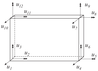
|
planre |
Compute element matrices |
planrs |
Compute section forces |
platre
- Purpose:
Compute element stiffness matrix for a rectangular plate element.

- Syntax:
Ke = platre(ex, ey, ep, D) [Ke, fe] = platre(ex, ey, ep, D, eq)- Description:
platreprovides an element stiffness matrix \(Ke\), and an element load vector \(fe\), for a rectangular plate element. This element can only be used if the element edges are parallel to the coordinate axes.The element nodal coordinates \(x_1, y_1, x_2\) etc. are supplied to the function by \(\mathbf{ex}\) and \(\mathbf{ey}\), the element thickness \(t\) by \(\mathbf{ep}\), and the material properties by the constitutive matrix \(D\). Any arbitrary \(\mathbf{D}\)-matrix with dimensions \((3 \times 3)\) and valid for plane stress may be given. For an isotropic elastic material the constitutive matrix can be formed by the function
hooke(see Section Material functions).\[\begin{split}\begin{array}{l} \mathbf{ex} = [\, x_1 \;\; x_2 \;\; x_3 \;\; x_4 \,] \\ \mathbf{ey} = [\, y_1 \;\; y_2 \;\; y_3 \;\; y_4 \,] \end{array} \qquad \mathbf{ep} = [\, t \,] \qquad \mathbf{D} = \begin{bmatrix} D_{11} & D_{12} & D_{13} \\ D_{21} & D_{22} & D_{23} \\ D_{31} & D_{32} & D_{33} \end{bmatrix}\end{split}\]If a uniformly distributed load is applied to the element, the element load vector \(fe\) is computed. The input variable
\[\mathbf{eq} = [\, q_z \,]\]then contains the load \(q_z\) per unit area in the \(z\)-direction.
- Theory:
The element stiffness matrix \(\mathbf{K}^e\) and the element load vector \(\mathbf{f}_l^e\), stored in \(Ke\) and \(fe\) respectively, are computed according to
\[\mathbf{K}^e = (\mathbf{C}^{-1})^T \int_A \bar{\mathbf{B}}^T \tilde{\mathbf{D}} \, \bar{\mathbf{B}} \, dA \, \mathbf{C}^{-1}\]\[\mathbf{f}_l^e = (\mathbf{C}^{-1})^T \int_A \bar{\mathbf{N}}^T q_z \, dA\]where the constitutive matrix
\[\tilde{\mathbf{D}} = \frac{t^3}{12} \mathbf{D}\]and where \(\mathbf{D}\) is defined by \(D\).
The evaluation of the integrals for the rectangular plate element is based on the displacement approximation \(w(x, y)\) and is expressed in terms of the nodal variables \(u_1, u_2, \ldots, u_{12}\) as
\[w(x, y) = \mathbf{N}^e \mathbf{a}^e = \bar{\mathbf{N}} \mathbf{C}^{-1} \mathbf{a}^e\]where
\[\bar{\mathbf{N}} = [\, 1 \;\; x \;\; y \;\; x^2 \;\; x y \;\; y^2 \;\; x^3 \;\; x^2 y \;\; x y^2 \;\; y^3 \;\; x^3 y \;\; x y^3 \,]\]\[\begin{split}\mathbf{C} = \left[ \begin{array}{cccccccccccc} 1 & -a & -b & a^2 & ab & b^2 & -a^3 & -a^2b & -ab^2 & -b^3 & a^3b & ab^3 \\ 0 & 0 & 1 & 0 & -a & -2b & 0 & a^2 & 2ab & 3b^2 & -a^3 & -3ab^2 \\ 0 & -1 & 0 & 2a & b & 0 & -3a^2 & -2ab & -b^2 & 0 & 3a^2b & b^3 \\ 1 & a & -b & a^2 & -ab & b^2 & a^3 & -a^2b & ab^2 & -b^3 & -a^3b & -ab^3 \\ 0 & 0 & 1 & 0 & a & -2b & 0 & a^2 & -2ab & 3b^2 & a^3 & 3ab^2 \\ 0 & -1 & 0 & -2a & b & 0 & -3a^2 & 2ab & -b^2 & 0 & 3a^2b & b^3 \\ 1 & a & b & a^2 & ab & b^2 & a^3 & a^2b & ab^2 & b^3 & a^3b & ab^3 \\ 0 & 0 & 1 & 0 & a & 2b & 0 & a^2 & 2ab & 3b^2 & a^3 & 3ab^2 \\ 0 & -1 & 0 & -2a & -b & 0 & -3a^2 & -2ab & -b^2 & 0 & -3a^2b & -b^3 \\ 1 & -a & b & a^2 & -ab & b^2 & -a^3 & a^2b & -ab^2 & b^3 & -a^3b & -ab^3 \\ 0 & 0 & 1 & 0 & -a & 2b & 0 & a^2 & -2ab & 3b^2 & -a^3 & -3ab^2 \\ 0 & -1 & 0 & 2a & -b & 0 & -3a^2 & 2ab & -b^2 & 0 & -3a^2b & -b^3 \end{array} \right]\end{split}\]\[\mathbf{a}^e = [\, u_1 \;\; u_2 \;\; \ldots \;\; u_{12} \,]^T\]and where
\[a = \frac{1}{2}(x_3 - x_1) \qquad b = \frac{1}{2}(y_3 - y_1)\]The matrix \(\bar{\mathbf{B}}\) is obtained as
\[\begin{split}\bar{\mathbf{B}} = \stackrel{*}{\nabla} \bar{\mathbf{N}} = \left[ \begin{array}{cccccccccccc} 0 & 0 & 0 & 2 & 0 & 0 & 6x & 2y & 0 & 0 & 6xy & 0 \\ 0 & 0 & 0 & 0 & 0 & 2 & 0 & 0 & 2x & 6y & 0 & 6xy \\ 0 & 0 & 0 & 0 & 2 & 0 & 0 & 4x & 4y & 0 & 6x^2 & 6y^2 \\ \end{array} \right]\end{split}\]where
\[\begin{split}\stackrel{*}{\nabla} = \begin{bmatrix} \frac{\partial^2}{\partial x^2} \\ \frac{\partial^2}{\partial y^2} \\ 2 \frac{\partial^2}{\partial x \partial y} \end{bmatrix}\end{split}\]Evaluation of the integrals for the rectangular plate element is done analytically. Computation of the integrals for the element load vector \(\mathbf{f}_l^e\) yields
\[\begin{split}\mathbf{f}_l^e = q_z L_x L_y \begin{bmatrix} \frac{1}{4} \\ \frac{L_y}{24} \\ -\frac{L_x}{24} \\ \frac{1}{4} \\ \frac{L_y}{24} \\ \frac{L_x}{24} \\ \frac{1}{4} \\ -\frac{L_y}{24} \\ \frac{L_x}{24} \\ \frac{1}{4} \\ -\frac{L_y}{24} \\ -\frac{L_x}{24} \end{bmatrix}\end{split}\]where
\[L_x = x_3 - x_1 \qquad L_y = y_3 - y_1\]
platrs
- Purpose:
Compute section forces in a rectangular plate element.

- Syntax:
[es,et]=platrs(ex,ey,ep,D,ed)- Description:
\(\mathtt{platrs}\) computes the section forces \(\mathtt{es}\) and the curvature matrix \(\mathtt{et}\) in a rectangular plate element. The section forces and the curvatures are computed at the center of the element.
The input variables \(\mathbf{ex}\), \(\mathbf{ey}\), \(\mathbf{ep}\) and \(\mathbf{D}\) are defined in \(\mathtt{platre}\). The vector \(\mathbf{ed}\) contains the nodal displacements \(\mathbf{a}^e\) of the element and is obtained by the function \(\mathtt{extract}\) as
\[\mathbf{ed} = (\mathbf{a}^e)^T = [\,u_1\;\; u_2\;\; \ldots \;\; u_{12}\;]\]The output variables
\[\mathtt{es} = \left[\,\mathbf{M}^T\; \mathbf{V}^T\,\right] = \left[\, M_{xx}\; M_{yy}\; M_{xy}\; V_{xz}\; V_{yz}\; \right]\]\[\mathtt{et} = \boldsymbol{\kappa}^T = \left[\, \kappa_{xx}\; \kappa_{yy}\; \kappa_{xy}\; \right]\]contain the section forces and curvatures in global directions.
- Theory:
The curvatures and the section forces are computed according to
\[\begin{split}\boldsymbol{\kappa} = \left[ \begin{array}{c} \kappa_{xx} \\ \kappa_{yy} \\ \kappa_{xy} \end{array} \right] = \bar{\mathbf{B}}\,\mathbf{C}^{-1}\,\mathbf{a}^e\end{split}\]\[\begin{split}\mathbf{M} = \left[ \begin{array}{c} M_{xx} \\ M_{yy} \\ M_{xy} \end{array} \right] = \tilde{\mathbf{D}}\,\boldsymbol{\kappa}\end{split}\]\[\begin{split}\mathbf{V} = \left[ \begin{array}{c} V_{xz} \\ V_{yz} \end{array} \right] = \tilde{\nabla}\,\mathbf{M}\end{split}\]where the matrices \(\tilde{\mathbf{D}}\), \(\bar{\mathbf{B}}\), \(\mathbf{C}\) and \(\mathbf{a}^e\) are described in \(\mathtt{platre}\), and where
\[\begin{split}\tilde{\nabla} = \left[ \begin{array}{ccc} \dfrac{\partial}{\partial x} & 0 & \dfrac{\partial}{\partial y} \\ 0 & \dfrac{\partial}{\partial y} & \dfrac{\partial}{\partial x} \end{array} \right]\end{split}\]