exs_spring
- Purpose:
Show the basic steps in a finite element calculation.
- Description:
The general procedure in linear finite element calculations is carried out for a simple structure. The steps are:
Define the model
Generate element matrices
Assemble element matrices into the global system of equations
Solve the global system of equations
Evaluate element forces
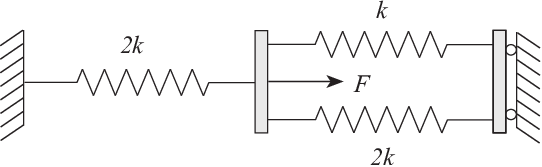
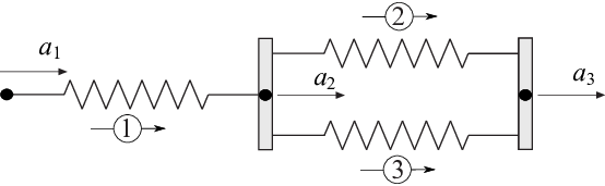
Consider the system of three linear elastic springs, and the corresponding finite element model. The system of springs is fixed in its ends and loaded by a single load \(F\).
- Example:
The computation is initialized by defining the topology matrix
Edof, containing element numbers and global element degrees of freedom:>> Edof=[1 1 2; 2 2 3; 3 2 3];The global stiffness matrix
K(3×3) of zeros:>> K=zeros(3,3) K = 0 0 0 0 0 0 0 0 0And the load vector
f(3×1) with the load \(F=100\) in position 2:>> f=zeros(3,1); f(2)=100 f = 0 100 0Element stiffness matrices are generated by the function
spring1e. The element propertyepfor the springs contains the spring stiffnesses \(k\) and \(2k\) respectively, where \(k=1500\):>> k=1500; ep1=2*k; ep2=k; ep3=2*k; >> Ke1=spring1e(ep1) Ke1 = 3000 -3000 -3000 3000 >> Ke2=spring1e(ep2) Ke2 = 1500 -1500 -1500 1500 >> Ke3=spring1e(ep3) Ke1 = 3000 -3000 -3000 3000The element stiffness matrices are assembled into the global stiffness matrix
Kaccording to the topology:>> K=assem(Edof(1,:),K,Ke1) K = 3000 -3000 0 -3000 3000 0 0 0 0 >> K=assem(Edof(2,:),K,Ke2) K = 3000 -3000 0 -3000 4500 -1500 0 -1500 1500 >> K=assem(Edof(3,:),K,Ke3) K = 3000 -3000 0 -3000 7500 -4500 0 -4500 4500The global system of equations is solved considering the boundary conditions given in
bc:>> bc= [1 0; 3 0]; >> [a,r]=solveq(K,f,bc) a = 0 0.0133 0 r = -40.0000 0 -60.0000Element forces are evaluated from the element displacements. These are obtained from the global displacements
ausing the functionextract:>> ed1=extract_ed(Edof(1,:),a) ed1 = 0 0.0133 >> ed2=extract_ed(Edof(2,:),a) ed2 = 0.0133 0 >> ed3=extract_ed(Edof(3,:),a) ed3 = 0.0133 0The spring forces are evaluated using the function
spring1s:>> es1=spring1s(ep1,ed1) es1 = 40 >> es2=spring1s(ep2,ed2) es2 = -20 >> es3=spring1s(ep3,ed3) es3 = -40