exn_beam2g_b¶

Purpose:

Buckling analysis of a plane frame.

Description:

Buckling safety of the frame analysed in exn_beam2g is performed. The same computational model as in exn_beam2g is used. First, the same computation as in exn_beam2g is performed. In this computation the linear stiffness matrix is obtained by saving the stiffness matrix established using the function assem in the first iteration.

Example:

The computation follows the same procedure as in exn_beam2g, with the addition of topology, element properties, and coordinates definition:

import numpy as np
import calfem.core as cfc
import calfem.vis_mpl as cfv

edof = np.array([[4, 5, 6, 1, 2, 3], [7, 8, 9, 10, 11, 12], [4, 5, 6, 7, 8, 9]])

E = 200e9
A1 = 2e-3
A2 = 6e-3
I1 = 1.6e-5
I2 = 5.4e-5

ep1 = np.array([E, A1, I1])
ep3 = np.array([E, A2, I2])

ex1 = np.array([0.0, 0.0])
ey1 = np.array([4.0, 0.0])
ex2 = np.array([6.0, 6.0])
ey2 = np.array([4.0, 0.0])
ex3 = np.array([0.0, 6.0])
ey3 = np.array([4.0, 4.0])

eq1 = np.array([0.0])
eq2 = np.array([0.0])
eq3 = np.array([-50e3])

QX1 = 1e-4
QX2 = 0
QX3 = 0
QX01 = 1
eps = 1e-6
n = 0

During the iteration loop, the linear stiffness matrix is saved from the first iteration. The iteration proceeds until convergence:

while abs((QX1 - QX01) / QX01) > eps:
    n += 1
    K = np.zeros([12, 12])
    f = np.zeros([12, 1])
    f[3, 0] = 10e3

    Ke1 = cfc.beam2ge(ex1, ey1, ep1, QX1)
    Ke2 = cfc.beam2ge(ex2, ey2, ep1, QX2)
    Ke3, fe3 = cfc.beam2ge(ex3, ey3, ep3, QX3, eq3)

    K = cfc.assem(edof[0, :], K, Ke1)
    K = cfc.assem(edof[1, :], K, Ke2)
    K, f = cfc.assem(edof[2, :], K, Ke3, f, fe3)
    if n == 1:
        K0 = K

    bc = np.array([1, 2, 3, 10, 11])
    a, r = cfc.solveq(K, f, bc)

    ed = cfc.extract_ed(edof, a)

    QX01 = QX1
    es1 = cfc.beam2gs(ex1, ey1, ep1, ed[0, :], QX1, eq1)
    es2 = cfc.beam2gs(ex2, ey2, ep1, ed[1, :], QX2, eq2)
    es3 = cfc.beam2gs(ex3, ey3, ep3, ed[2, :], QX3, eq3)

    QX1 = es1[1]
    QX2 = es2[1]
    QX3 = es3[1]

    if n > 20:
        print("The solution does not converge")
        break

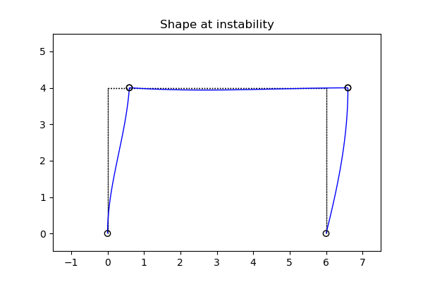
On the basis of the linear stiffness matrix \(\mathbf{K}_0\) and geometric nonlinear stiffness matrix \(\mathbf{K}_a\) obtained in that computation and stored in K0 and K, the generalised eigen value problem \((\mathbf{K}_a - \lambda \mathbf{K}_0)\phi = 0\) is established. Considering prescribed displacements specified in bc, the generalised eigen value problem is solved using eigen. Thereafter the loading factors corresponding to the buckling modes are computed as \(\alpha_i = \frac{1}{1 - \lambda_i}\):

lam, phi = cfc.eigen(K, K0, bc)
one = np.ones(lam.shape)
alpha = np.divide(one, one - lam)
print(alpha[0])

The loading factor corresponding to the first buckling mode is \(\alpha_1 = 6.89\). The shape at instability can be visualized using the first eigenvector:

Ed = cfc.extract_ed(edof, -phi[:, 0])
cfv.figure(1, fig_size=(6, 4))
plotpar = [3, 1, 0]
cfv.eldraw2(ex1, ey1, plotpar)
cfv.eldraw2(ex2, ey2, plotpar)
cfv.eldraw2(ex3, ey3, plotpar)
sfac = cfv.scalfact2(ex3, ey3, Ed[2, :], 0.1)
plotpar = [1, 2, 1]
cfv.eldisp2(ex1, ey1, Ed[0, :], plotpar, sfac)
cfv.eldisp2(ex2, ey2, Ed[1, :], plotpar, sfac)
cfv.eldisp2(ex3, ey3, Ed[2, :], plotpar, sfac)
cfv.plt.axis([-1.5, 7.5, -0.5, 5.5])
cfv.title("Shape at instability")
cfv.show_and_wait()