exn_beam2g
- Purpose:
Analysis of a plane frame considering geometric nonlinearity.
- Description:
The frame of
exs_beam2is analysed again, but it is now subjected to a load five times larger than inexs_beam2. Geometric nonlinearity is considered.The frame has the following properties: \(E=200\) GPa, \(A_1=2.0 \times 10^{-3}\) m², \(I_1=1.6 \times 10^{-5}\) m⁴, \(A_2=6.0 \times 10^{-3}\) m², \(I_2=5.4 \times 10^{-5}\) m⁴, \(P=10.0\) kN, and \(q_0=50.0\) kN/m. The corresponding computational model consists of three beam elements and twelve degrees of freedom.

- Example:
The computation is initialized by defining the topology matrix
edof, containing element numbers and global element degrees of freedom. The element property vectorsep1andep3, the element load vectorseq1,eq2andeq3, and the element coordinate vectorsex1,ex2,ex3,ey1,ey2, andey3are also defined:import numpy as np import calfem.core as cfc import calfem.vis_mpl as cfv edof = np.array([ [4, 5, 6, 1, 2, 3], [7, 8, 9, 10, 11, 12], [4, 5, 6, 7, 8, 9] ]) E = 200e9 A1 = 2e-3 A2 = 6e-3 I1 = 1.6e-5 I2 = 5.4e-5 ep1 = np.array([E, A1, I1]) ep3 = np.array([E, A2, I2]) ex1 = np.array([0.0, 0.0]) ey1 = np.array([4.0, 0.0]) ex2 = np.array([6.0, 6.0]) ey2 = np.array([4.0, 0.0]) ex3 = np.array([0.0, 6.0]) ey3 = np.array([4.0, 4.0]) eq1 = np.array([0.0]) eq2 = np.array([0.0]) eq3 = np.array([-50e3])The beam element function considering geometric nonlinearity
beam2gerequires the value of axial force \(Q_{\bar{x}}\). Since the axial forces are a result of the computation, the computation procedure is iterative. Initially, the axial forces are set to zero, i.e. \(Q_{\bar{x}}^{(1)}=0\), \(Q_{\bar{x}}^{(2)}=0\) and \(Q_{\bar{x}}^{(3)}=0\) which are stored inQX1,QX2andQX3. This means that the first iteration is equivalent to a linear analysis usingbeam2e. To make sure that the first iteration is performed, the scalar used for storing the previous axial force in Element 1QX01is set to 1. To avoid dividing by 0 in the second convergence check, a nonzero but small value is assumed for the initial axial force in Element 1, i.e. \(Q_{\bar{x}, 0}^{(1)}=1 \times 10^{-4}\). In each iteration the axial forcesQX1,QX2andQX3are updated according to the computational result. The iterations continue until the difference in axial forceQX1of the two latest iterations is less than an accepted errorepschosen as \(1.0 \times 10^{-6}\): (QX1-QX01) /QX01\(<\)eps:QX1 = 1e-4 QX2 = 0 QX3 = 0 QX01 = 1 eps = 1e-6 n = 0In each iteration the global stiffness matrix
K(12×12) and the load vectorf(12×1) are initially filled with zeros. The nodal load of 10.0 kN acting at upper left corner of the frame is placed in position 4 of the load vector. Element matrices are computed bybeam2geand assembled usingassem, after which the system of equations is solved usingsolveq. Based on the computed displacementsa, new values of section forces and axial forces are computed bybeam2gs. The axial forces are then extracted from the section force results. The first iteration’s element displacements are saved ined0for comparison with the linear analysis. IfQX1does not converge in 20 iterations the analysis is interrupted:while abs((QX1 - QX01) / QX01) > eps: n += 1 K = np.zeros([12, 12]) f = np.zeros([12, 1]) f[3, 0] = 10e3 Ke1 = cfc.beam2ge(ex1, ey1, ep1, QX1) Ke2 = cfc.beam2ge(ex2, ey2, ep1, QX2) Ke3, fe3 = cfc.beam2ge(ex3, ey3, ep3, QX3, eq3) K = cfc.assem(edof[0, :], K, Ke1) K = cfc.assem(edof[1, :], K, Ke2) K, f = cfc.assem(edof[2, :], K, Ke3, f, fe3) bc = np.array([1, 2, 3, 10, 11]) a, r = cfc.solveq(K, f, bc) ed = cfc.extract_ed(edof, a) QX01 = QX1 es1 = cfc.beam2gs(ex1, ey1, ep1, ed[0, :], QX1, eq1) es2 = cfc.beam2gs(ex2, ey2, ep1, ed[1, :], QX2, eq2) es3 = cfc.beam2gs(ex3, ey3, ep3, ed[2, :], QX3, eq3) QX1 = es1[1] QX2 = es2[1] QX3 = es3[1] if n == 1: ed0 = ed if n > 20: print("The solution does not converge") breakAfter convergence, section forces are computed for visualization with 21 evaluation points along each element:
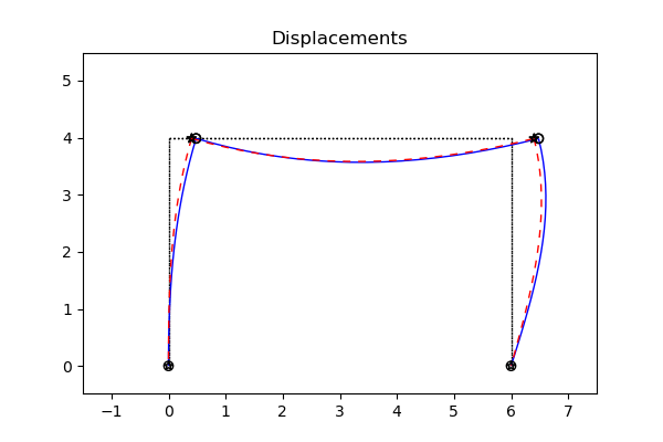
eq1 = np.array([0.0, eq1.item()])
eq2 = np.array([0.0, eq2.item()])
eq3 = np.array([0.0, eq3.item()])
es1, edi1, eci1 = cfc.beam2s(ex1, ey1, ep1, ed[0, :], eq1, 21)
es2, edi2, eci2 = cfc.beam2s(ex2, ey2, ep1, ed[1, :], eq2, 21)
es3, edi3, eci3 = cfc.beam2s(ex3, ey3, ep3, ed[2, :], eq3, 21)
eci1 = np.ravel(eci1)
eci2 = np.ravel(eci2)
eci3 = np.ravel(eci3)
A displacement diagram is displayed using the visualization module. The deformed frame is shown with both the linear analysis result (from the first iteration) and the nonlinear analysis result:
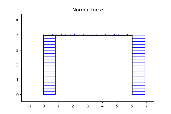
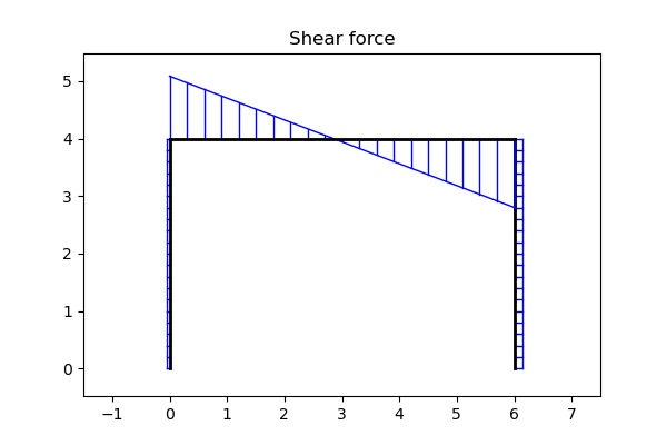
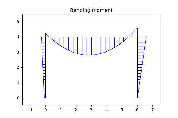
cfv.figure(1, fig_size=(6, 4))
plotpar = [3, 1, 0]
cfv.eldraw2(ex1, ey1, plotpar)
cfv.eldraw2(ex2, ey2, plotpar)
cfv.eldraw2(ex3, ey3, plotpar)
sfac = cfv.scalfact2(ex3, ey3, edi3, 0.1)
plotpar = [1, 2, 1]
cfv.eldisp2(ex1, ey1, ed[0, :], plotpar, sfac)
cfv.eldisp2(ex2, ey2, ed[1, :], plotpar, sfac)
cfv.eldisp2(ex3, ey3, ed[2, :], plotpar, sfac)
plotpar = [2, 4, 2]
cfv.eldisp2(ex1, ey1, ed0[0, :], plotpar, sfac)
cfv.eldisp2(ex2, ey2, ed0[1, :], plotpar, sfac)
cfv.eldisp2(ex3, ey3, ed0[2, :], plotpar, sfac)
cfv.plt.axis([-1.5, 7.5, -0.5, 5.5])
cfv.title("Displacements")
Section force diagrams (normal force, shear force, and bending moment) can also be displayed:
# Normal force diagram
cfv.figure(2, fig_size=(6, 4))
plotpar = [2, 1]
sfac = cfv.scalfact2(ex1, ey1, es1[:, 0], 0.2)
cfv.secforce2(ex1, ey1, es1[:, 0], plotpar, sfac, eci1)
cfv.secforce2(ex2, ey2, es2[:, 0], plotpar, sfac, eci2)
cfv.secforce2(ex3, ey3, es3[:, 0], plotpar, sfac, eci3)
cfv.plt.axis([-1.5, 7.5, -0.5, 5.5])
cfv.title("Normal force")

# Shear force diagram
cfv.figure(3, fig_size=(6, 4))
plotpar = [2, 1]
sfac = cfv.scalfact2(ex3, ey3, es3[:, 1], 0.2)
cfv.secforce2(ex1, ey1, es1[:, 1], plotpar, sfac, eci1)
cfv.secforce2(ex2, ey2, es2[:, 1], plotpar, sfac, eci2)
cfv.secforce2(ex3, ey3, es3[:, 1], plotpar, sfac, eci3)
cfv.plt.axis([-1.5, 7.5, -0.5, 5.5])
cfv.title("Shear force")

# Bending moment diagram
cfv.figure(4, fig_size=(6, 4))
plotpar = [2, 1]
sfac = cfv.scalfact2(ex3, ey3, es3[:, 2], 0.2)
cfv.secforce2(ex1, ey1, es1[:, 2], plotpar, sfac, eci1)
cfv.secforce2(ex2, ey2, es2[:, 2], plotpar, sfac, eci2)
cfv.secforce2(ex3, ey3, es3[:, 2], plotpar, sfac, eci3)
cfv.plt.axis([-1.5, 7.5, -0.5, 5.5])
cfv.title("Bending moment")
cfv.show_and_wait()